Chapter 6 Risk Prediction and Validation (Part II)
6.1 The Brier Score
Binary outcomes - \(Y_{i}\) for individual \(i\).
Let \(g(\mathbf{x}_{i})\) be a risk score for an individual with covariate vector \(\mathbf{x}_{i}\).
If \(g(\mathbf{x}_{i})\) is interpreted as an estimate of the probability that \(Y_{i} = 1\), the Brier score is a measure of the predictive accuracy of \(g(\mathbf{x}_{i})\).
For binary outcomes \(Y_{i}\) and risk scores \(g(\mathbf{x}_{i})\), the Brier score is defined as \[\begin{equation} BS(Y, g) = \frac{1}{n}\sum_{i=1}^{n} \{ Y_{i} - g(\mathbf{x}_{i}) \}^{2} \end{equation}\]
The Brier score is typically used to compare the accuracy of risk scores.
- It is hard to tell if a risk score is good just by looking at the Brier score itself without comparing it with other methods.
- Even if \(g(\mathbf{x}_{i})\) is a class prediction rather than a probability (i.e., \(g(\mathbf{x}_{i}) = 0\) or \(g(\mathbf{x}_{i}) = 1\)), the Brier score can be interpreted as the proportion of “misclassified” outcomes \[\begin{equation} BS(Y, g) = \frac{1}{n}\sum_{i=1}^{n} \{ Y_{i} - g(\mathbf{x}_{i}) \}^{2} = \frac{1}{n} \sum_{i=1}^{n} I\{Y_{i} \neq g(\mathbf{x}_{i}) \} \end{equation}\]
The Brier score is a single measure that is affected by both the discrimination and calibration of the risk score.
The usual justification for this is to look at the following approximation of the Brier score \[\begin{equation} BS(Y, g) \approx \tilde{BS}(Y,g) = \frac{1}{n}\sum_{s=1}^{S} \sum_{i=1}^{n} a_{is}\{Y_{i} - \bar{g}_{s} \}^{2} \end{equation}\]
This approximation assumes \(S\) strata: \([s_{0}, s_{1}), [s_{1}, s_{2}), \ldots, [s_{S-1}, s_{S})\).
\(a_{is}\) is an indicator of whether or not the \(i^{th}\) observation falls into the \(s^{th}\) stratum:
- That is, \(a_{is} = 1\) if \(s_{s-1} \leq g(\mathbf{x}_{i}) < s_{s}\)
\(\bar{g}_{s}\) is the average value of the risk score within stratum \(s\) \[\begin{equation} \bar{g}_{s} = \frac{1}{n_{s}} \sum_{i=1}^{n} a_{is} g(\mathbf{x}_{i}) \end{equation}\] and \(n_{s}\) is the number of observation where the risk score is in stratum \(s\).
- If we let \(\bar{Y}_{s} = \frac{1}{n_{s}}\sum_{i=1}^{n} a_{is}Y_{i}\) be the proportion of 1’s in stratum \(s\), we can simplify the expression for the approximate Brier score as follows: \[\begin{eqnarray} \tilde{BS}(Y,g) &=& \frac{1}{n}\sum_{s=1}^{S} \sum_{i=1}^{n} a_{is}\{Y_{i} - \bar{Y}_{s} + \bar{Y}_{s} - \bar{g}_{s} \}^{2} \nonumber \\ &=& \frac{1}{n}\sum_{s=1}^{S} \sum_{i=1}^{n} a_{is}\{Y_{i} - \bar{Y}_{s} \}^{2} + \frac{1}{n}\sum_{s=1}^{S} n_{s}\{\bar{Y}_{s} - \bar{g}_{s} \}^{2} \nonumber \\ &=& \frac{1}{n}\sum_{s=1}^{S} n_{s}\bar{Y}_{s}(1 - \bar{Y}_{s}) + \frac{1}{n}\sum_{s=1}^{S} n_{s}\{\bar{Y}_{s} - \bar{g}_{s} \}^{2} \nonumber \\ &=& B_{D} + B_{C} \end{eqnarray}\]
The quantity \(B_{D} = \frac{1}{n}\sum_{s=1}^{S} n_{s}\bar{Y}_{s}(1 - \bar{Y}_{s})\) is related to the discrimination of the risk score \(g\).
To get a sense of why \(B_{D}\) measures discrimination, suppose \(s\) is a stratum where \(s_{s} \leq t\).
If the risk score has good discrimination, this threshold should separate most of the “successes” from the “failures”.
- That is most with \(g(\mathbf{x}_{i}) \leq t\) has \(Y_{i} = 0\) and most with \(g(\mathbf{x}_{i}) > t\) has \(Y_{i}=1\).
- This \(\bar{Y}_{s}(1 - \bar{Y}_{s})\) is close to \(0\).
- If this is close to \(0\) for most threholds, \(B_{D}\) will be small.
The quantity \(B_{C} = \frac{1}{n}\sum_{s=1}^{S} n_{s}\{\bar{Y}_{s} - \bar{g}_{s} \}^{2}\) is a measure of calibration.
For a well-calibrated risk score, the proportion of successes \(\bar{Y}_{s}\) in stratum \(s\) should be close to the average value of the risk score \(g_{s}\) in stratum \(s\).
6.1.1 Brier scores for biopsy data
- Let’s compute the Brier score using the
biopsydata again from theMASSpackage.
library(rpart)
library(MASS)

data(biopsy)
# Create binary outcome for tumor class
biopsy$tumor.type <- ifelse(biopsy$class=="malignant", 1, 0)
head(biopsy)
## ID V1 V2 V3 V4 V5 V6 V7 V8 V9 class tumor.type
## 1 1000025 5 1 1 1 2 1 3 1 1 benign 0
## 2 1002945 5 4 4 5 7 10 3 2 1 benign 0
## 3 1015425 3 1 1 1 2 2 3 1 1 benign 0
## 4 1016277 6 8 8 1 3 4 3 7 1 benign 0
## 5 1017023 4 1 1 3 2 1 3 1 1 benign 0
## 6 1017122 8 10 10 8 7 10 9 7 1 malignant 1- Let’s try constructing fitted probabilities using three approaches:
- logistic regression
- CART
- random forest
library(rpart)
library(randomForest)

# Fit CART, logistic regression, and random forest
cart.model <- rpart(class ~ V1 + V3 + V4 + V7 + V8, data=biopsy)
logreg.model <- glm(tumor.type ~ V1 + V3 + V4 + V7 + V8, family="binomial", data=biopsy)
RF.model <- randomForest(class ~ V1 + V3 + V4 + V7 + V8, data=biopsy, ntree = 500)- Let’s then compute “risk scores” from each method.
##      benign malignant
## 1 0.9837587 0.0162413
## 2 0.0952381 0.9047619
## 3 0.9837587 0.0162413
## 4 0.0952381 0.9047619
## 5 0.9837587 0.0162413
## 6 0.0952381 0.9047619
# We want the second column of this matrix for the CART fitted probabilities
risk.cart <- probs.cart[,2]
# logistic regression
risk.logreg <- predict(logreg.model, newdata=biopsy, type="response")
# random forest risk scores
risk.RF <- predict(RF.model, newdata=biopsy, type = "prob")[,2]- The in-sample Brier scores for each method are:
- “In-sample” here meaning we are computing the Brier score using the same outcomes we used to construct the risk scores.
brier.cart <- mean((risk.cart - biopsy$tumor.type)^2)
brier.logreg <- mean((risk.logreg - biopsy$tumor.type)^2)
brier.RF <- mean((risk.RF - biopsy$tumor.type)^2)

round(c(brier.cart, brier.logreg, brier.RF), 4)
## [1] 0.0450 0.0280 0.0056- When comparing in-sample Brier scores, CART is the worst, logistic regression is in the middle, and random forest is the best.
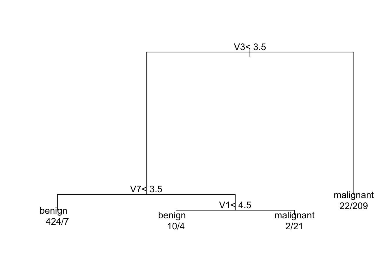
Figure 6.1: Fitted CART model for the biopsy data
6.1.2 Out-of-sample comparisons
Looking at out-of-sample performance is a better way to validate our risk scores.
Let’s try a validation exercise by “training” our models on the first \(400\) observations of
biopsyand then testing relative performance on the remaining observations.
# Create train/test splits for biopsy data
biopsy.train <- biopsy[1:400,]
biopsy.test <- biopsy[401:699,]
# Now, use each type of method on this training data
cart.model.train <- rpart(class ~ V1 + V3 + V4 + V7 + V8, data=biopsy.train)
logreg.model.train <- glm(tumor.type ~ V1 + V3 + V4 + V7 + V8, family="binomial",
data=biopsy.train)
RF.model.train <- randomForest(class ~ V1 + V3 + V4 + V7 + V8, data=biopsy.train,
ntree = 500)- Using these models built on the training data, get the fitted probabilities for the test data
risk.cart.test <- predict(cart.model.train, newdata=biopsy.test)[,2]
risk.logreg.test <- predict(logreg.model.train, newdata=biopsy.test, type="response")
risk.RF.test <- predict(RF.model.train, newdata=biopsy.test, type = "prob")[,2]- Now, using these fitted probabilities on the test data, compute the Brier scores:
brier.cart.test <- mean((risk.cart.test - biopsy.test$tumor.type)^2)
brier.logreg.test <- mean((risk.logreg.test - biopsy.test$tumor.type)^2)
brier.RF.test <- mean((risk.RF.test - biopsy.test$tumor.type)^2)

round(c(brier.cart.test, brier.logreg.test, brier.RF.test), 4)
## [1] 0.0359 0.0135 0.0183For the out-of-sample Brier score, both logistic regression and random forest are notably better than CART.
Logistic regression is actually slightly better than random forest in out of sample performance with random forest (at least for this particular train/test split).
6.2 Brier Scores with Survival Data
In survival analysis, we have random variables \(T_{1}, \ldots, T_{n}\) which represent times until
Due to right-censoring, we only observe pairs: \((U_i, \delta_i)\), where
- \(U_i = \min(T_{i}, C_{i})\) is the last follow-up time
- \(\delta_i = I(T_{i} \leq C_{i})\) is the event indicator
- \(C_{i}\) - censoring time
Suppose we could observe the survival times \(T_{i}\).
If we could observe \(T_{i}\), we could define the following binary variables (for a pre-specified value of \(t\)). \[\begin{equation} Y_i(t) = I(T_i > t) \end{equation}\]
\(Y_i(t) = 1\): Subject is alive at time \(t\).
\(Y_i(t) = 0\): Subject has experienced the event by time \(t\).
If we could observe \(T_{i}\), we could use the same form of the Brier score as for binary outcomes: \[\begin{align} BS_{\textrm{naive}}(t; S) &= \frac{1}{n} \sum_{i=1}^{n} \Big( Y_{i}(t) - P\{Y_{i}(t)=1 | \mathbf{x}_{i} \} \Big)^2 \nonumber \\ &= \frac{1}{n} \sum_{i=1}^{n} \Big( I(T_{i} > t) - S(t|\mathbf{x}_{i}) \Big)^2 \end{align}\]
\(\hat{S}(t|\mathbf{x}_{i}) = P(T_{i} > t| \mathbf{x}_{i})\): survival probability given covariates.
The main problem with using the above “naive” Brier score is that we cannot usually create this binary outcomes in the presence of right censoring.
- For example, if subject \(i\) is censored at time \(C_i < t\), we do not know if they are alive or dead at time \(t\).
Solution use a weighted version of the naive Brier score with weights based on Inverse Probability of Censoring Weighting (IPCW).
Weights are derived from the censoring distribution \(G(t) = P(C > t)\) (usually estimated via Kaplan-Meier on the censoring times).
With IPCW, the Brier score is \[\begin{equation} BS(t; S) = \frac{1}{n} \sum_{i=1}^{n} W_{i}(t)\Big( I(U_{i} > t) - S(t|\mathbf{x}_{i}) \Big)^2 \end{equation}\] where the weights are \[\begin{equation} W_{i}(t) = \frac{I(U_{i} \leq t)\delta_{i}}{ G(T_{i})} + \frac{I(U_{i} > t)}{G(t)} \end{equation}\]
Unlike with binary outcomes, the survival Brier score depends on a particular choice of \(t\).
You can plot the Brier score as a function of \(t\) to get a sense of how it changes over time:
Plotting \(BS(t, S)\) as a function of \(t\) is useful for comparing models and to see when the model has worse performance
- Does it fail to predict early mortality?
- Does it lose calibration at long-term follow-up?
- The Integrated Brier Score (IBS) gives you a **single summary measures for the entire study period, we integrate the area under the Brier Score curve.
\[IBS = \frac{1}{\tau} \int_0^\tau BS(t) dt\]
- \(\tau\): The time horizon of interest (e.g., 5 years).
- Often \(\tau\) is near the last censoring time.
- Benchmark: As a rough benchmark, you can compare your Brier score with
the Brier score from a single Kaplan-Meier estimator.
- You want your covariate-dependent survival model to perform at least noticeably better than the single Kaplan-Meier estimator.
\[\begin{equation} BS(t; S_{KM}) = \frac{1}{n} \sum_{i=1}^{n} W_{i}(t)\Big( Y_{i}(t) - S_{KM}(t) \Big)^2 \end{equation}\]
6.3 The integrated Brier score in R
The SurvMetrics package directly computes the integrated Brier score.
library(survival)
library(SurvMetrics)

df <- na.omit(lung)

# 1. Fit the Model
fit_cox <- coxph(Surv(time, status) ~ age + sex, data = df)

# 2. Define Time Points
time_points <- seq(100, 800, by = 100)

# 3. Manually extract the predicted survival probability matrix
# summary() with survfit returns a matrix of dimensions [times, patients]
surv_data <- summary(survfit(fit_cox, newdata = df), times = time_points)

# Transpose it so Rows = Patients and Cols = Times (Required by SurvMetrics)
sp_matrix <- t(surv_data$surv)

# 4. Calculate IBS
# Pass the true Surv object, the probability matrix, and the time vector
ibs_value <- IBS(object = Surv(df$time, df$status),
                 sp_matrix = sp_matrix,
                 IBSrange = time_points)

print(ibs_value)
## IBS
## 0.5013186.4 Brier Scores with Longitudinal Data
- Let’s revisit the
ohiodata again from thegeepackpackage
##    resp id age smoke
## 1     0  0  -2     0
## 2     0  0  -1     0
## 3     0  0   0     0
## 4     0  0   1     0
## 5     0  1  -2     0
## 6     0  1  -1     0
## 7     0  1   0     0
## 8     0  1   1     0
## 9     0  2  -2     0
## 10    0  2  -1     0
Each individual has 4 follow-up visits.
The variable
respis the wheezing status of the individual at each follow up.The variable
smokeis a baseline variable that does not change over time. This is an indicator of maternal smoking.ageis a time-varying covariate.
6.4.1 Option 1
If we want to build a risk score for wheezing, evaluating the performance of this risk score will depend on exactly what we are trying to predict.
Option 1: We want to predict whether or not some someone is diagnosed with wheezing over some time window, and we do not want to predict wheezing status at each time point.
As an example of this, let’s build a risk score which:
Only uses
smokeas a covariate.Builds the risk score from the first two follow-up times.
- Let’s first construct a dataset called
atleastone1that records whether or not an individual had at least one positive wheezing status over the first two visits:atleastone2will record whether or not an individual has at least one positive wheezing status over the last two visits.
data(ohio)
baseline.ohio <- subset(ohio, age== -1) # data from baseline visit
firsttwo.ohio <- subset(ohio, age== -1 | age == 0) # data from visits 1-2
lasttwo.ohio <- subset(ohio, age==1 | age==2) # data from visits 3-4

tmp <- aggregate(firsttwo.ohio$resp, by=list(id=firsttwo.ohio$id), FUN=max)
tmp2 <- aggregate(lasttwo.ohio$resp, by=list(id=lasttwo.ohio$id), FUN=max)
atleastone1 <- merge(tmp, baseline.ohio, by="id")
atleastone2 <- merge(tmp2, baseline.ohio, by="id")
head(atleastone1)
## id x resp age smoke
## 1 0 0 0 -1 0
## 2 1 0 0 -1 0
## 3 2 0 0 -1 0
## 4 3 0 0 -1 0
## 5 4 0 0 -1 0
## 6 5 0 0 -1 0##
## 0 1
## 446 91- Let’s now build a risk score using only variable
smokeas a covariate and a random choice of \(300\) observations
set.seed(1234)
train.ind <- sample(1:537, size=300)
atleastone1.train <- atleastone1[train.ind,]
mod1 <- glm(resp ~ smoke, family="binomial", data=atleastone1.train)
summary(mod1)
##
## Call:
## glm(formula = resp ~ smoke, family = "binomial", data = atleastone1.train)
##
## Coefficients:
## Estimate Std. Error z value Pr(>|z|)
## (Intercept) -1.7979 0.2078 -8.653 <2e-16 ***
## smoke 0.1665 0.3311 0.503 0.615
## ---
## Signif. codes: 0 '***' 0.001 '**' 0.01 '*' 0.05 '.' 0.1 ' ' 1
##
## (Dispersion parameter for binomial family taken to be 1)
##
## Null deviance: 253.63 on 299 degrees of freedom
## Residual deviance: 253.37 on 298 degrees of freedom
## AIC: 257.37
##
## Number of Fisher Scoring iterations: 4- The risk scores for the hold-out individuals for the later follow-up times are given by
- Now, let’s look at the Brier score on the remaining individuals in the
atleast2data set.
## [1] 0.1574466An AUC probably does not make much sense here since there are only two possible values of the risk score.
For calibration, we can just compare the predicted risk scores and the mean number of successes in each of the smoking categories in the hold-out sample:
## risk1
## 0.142105263157904 0.163636363636364
## 160 77##
## 0 1
## 0 135 56
## 1 25 21## [1] 0.15625## [1] 0.2727273- This risk score does not seem all that well-calibrated for later time points.
- The overall prevalence of wheezing is a little bit higher in the hold-out sample.
- There is a larger difference between the smoking and non-smoking groups in the hold-out sample.
6.4.2 Option 2
As another option, you may want to predict outcomes for each time point in the hold-out dataset.
In this case, I would probably just compute a Brier score by just averaging over all time points.
For example, with a GEE, you might do the following:
ind <- c(1:400, 801:1200, 1601:2000) ## index of training set
ohio.train <- subset(ohio[ind,], age==-1 | age == 0)
ohio.test <- subset(ohio[-ind,], age==1 | age==2)
fit.ex <- geeglm(resp ~ age + smoke + age:smoke, id=id, data=ohio.train,
                 family=binomial, corstr="exch")
rs2 <- predict(fit.ex, newdata=ohio.test, type="response")

## Now, find Brier score that the takes average across all individuals and time points
mean((rs2 - ohio.test$resp)^2)
## [1] 0.1270949