Chapter 5 Risk Prediction and Validation (Part I)

---

5.1 Risk Prediction/Stratification

• For binary outcomes, a risk prediction is related to the predicted probability that an individual has or will develop a certain condition/trait.

• Examples of a risk prediction for a binary outcome:

  • Probability that someone has hypertension.

  • Probability that someone has type-2 diabetes.

  • Probability someone will be hospitalized over the next 1 year.

• Risk stratification: Often, a risk prediction model will only report whether or not someone belongs to one of several risk strata.

  • For example, high, medium, or low risk.

5.2 Area under the ROC curve and the C-statistic

5.2.1 Sensitivity and Specificity

• Let $g(\mathbf{x}_{i})$ be a risk score for an individual with covariate vector $\mathbf{x}_{i}$.

• Higher values of $g(\mathbf{x}_{i})$ are supposed to imply greater probability that the binary outcome $Y_{i}$ is equal to $1$.

  • Though $g(\mathbf{x}_{i})$ does not necessarily have to be a predicted probability.

• The value $t$ will be a threshold which determines whether or not, we predict $Y_{i} = 1$ or not.

  • $g(\mathbf{x}_{i}) \geq t$ implies $Y_{i} = 1$
  • $g(\mathbf{x}_{i}) < t$ implies $Y_{i} = 0$

---

• The sensitivity of the risk score $g(\mathbf{x}_{i})$ with the threshold $t$ is defined as the probability you “predict” $Y_{i} = 1$ assuming that $Y_{i}$ is, in fact, equal to $1$.

• In other words, the sensitivity is the probability of making the right decision given that $Y_{i} = 1$.

  • Sensitivity is often called the “true positive rate”.

• The sensitivity is defined as: $$\begin{eqnarray} \textrm{Sensitivity}(t; g) &=& P\big\{ g(\mathbf{x}_{i}) \geq t| Y_{i} = 1 \big\} \nonumber \\ &=& \frac{P\big\{ g(\mathbf{x}_{i}) \geq t, Y_{i} = 1 \big\}}{P\big\{ Y_{i} = 1 \big\} }\nonumber \\ &=& \frac{P\big\{ g(\mathbf{x}_{i}) \geq t, Y_{i} = 1 \big\}}{ P\big\{ g(\mathbf{x}_{i}) \geq t, Y_{i} = 1 \big\} + P\big\{ g(\mathbf{x}_{i}) < t, Y_{i} = 1 \big\}} \end{eqnarray}$$

• For a worthless risk score that is totally uninformative about the outcome, we should expect the sensitivity to be close to $P\{ g(\mathbf{x}_{i}) \geq t \}$.

---

• You can compute the in-sample sensitivity with $$\begin{eqnarray} \hat{\textrm{Sensitivity}}(t; g) &=& \frac{\sum_{i=1}^{n} I\big\{ g(\mathbf{x}_{i}) \geq t, Y_{i} = 1 \big\} }{ \sum_{i=1}^{n} I\big\{g(\mathbf{x}_{i}) \geq t, Y_{i} = 1 \big\} + \sum_{i=1}^{n} I\big\{ g(\mathbf{x}_{i}) < t, Y_{i} = 1 \big\}} \nonumber \\ &=& \frac{\textrm{number of true positives}}{\textrm{number of true positives} + \textrm{number of false negatives} } \end{eqnarray}$$

---

• The specificity of the risk score $g(\mathbf{x}_{i})$ with the threshold $t$ is defined as the probability you “predict” $Y_{i} = 0$ assuming that $Y_{i}$ is, in fact, equal to $0$.

• The specificity is defined as: $$\begin{eqnarray} \textrm{Specificity}(t; g) &=& P\big\{ g(\mathbf{x}_{i}) < t| Y_{i} = 0 \big\} \nonumber \\ &=& \frac{P\big\{ g(\mathbf{x}_{i}) < t, Y_{i} = 0 \big\}}{ P\big\{ g(\mathbf{x}_{i}) < t, Y_{i} = 0 \big\} + P\big\{ g(\mathbf{x}_{i}) \geq t, Y_{i} = 0 \big\}} \end{eqnarray}$$

• Note that $1 - \textrm{Specificity}(t; g) = P\big\{ g(\mathbf{x}_{i}) \geq t| Y_{i} = 0 \big\}$.

  • $1 - \textrm{Specificity}(t; g)$ is often called the “false positive rate”

---

• You can compute the in-sample specificity with $$\begin{eqnarray} \hat{\textrm{Specificity}}(t; g) &=& \frac{\sum_{i=1}^{n} I\big\{ g(\mathbf{x}_{i}) < t, Y_{i} = 0 \big\} }{ \sum_{i=1}^{n} I\big\{g(\mathbf{x}_{i}) < t, Y_{i} = 0 \big\} + \sum_{i=1}^{n} I\big\{ g(\mathbf{x}_{i}) \geq t, Y_{i} = 0 \big\}} \nonumber \\ &=& \frac{\textrm{number of true negatives}}{\textrm{number of true negatives} + \textrm{number of false positives} } \end{eqnarray}$$

• For a worthless risk score that is totally uninformative about the outcome, we should expect the specificity to be close to $P\{ g(\mathbf{x}_{i}) < t \}$.

• Note that high values of both sensitivity and specificity is good.

  • For a “perfect” risk score, both sensitivity and specificity would be equal to $1$.

5.2.2 The ROC curve

• The receiver operating characteristic (ROC) curve graphically depicts how sensitivity and specificity change as the threshold $t$ varies.

• Let $t_{i} = g(\mathbf{x}_{i})$ and let $t_{(1)} > t_{(2)} > ... > t_{(n)}$ be the ordered values of $t_{1}, \ldots, t_{n}$.

• To construct an ROC curve we are going to plot sentivity vs. 1 - specificity for each of the thresholds $t_{(1)}, \ldots, t_{(n)}$.

---

• Let $x_{i} = 1 - \hat{\textrm{Specificity}}(t_{(i)}; g)$ and $y_{i} = \hat{\textrm{Sensitivity}}(t_{(i)}; g)$.

• We will define $x_{0} = y_{0} = 0$ and $x_{n+1} = y_{n+1} = 1$.

  • $x_{0}$, $y_{0}$ represent 1 - specificity and sensitivity when using $t = \infty$.
  • $x_{n+1}$, $y_{n+1}$ represent 1 - specificity and sensitivity when using $t = -\infty$.

• Plotting $y_{i}$ vs. $x_{i}$ for $i = 0, \ldots, n+1$ will give you the ROC curve.

• Ideally, the values of $y_{i}$ will close to $1$ for all $i$.

• For a worthless risk score we should expect both $y_{i}$ and $x_{i}$ to be roughly equal to $P(g(\mathbf{x}_{i}) \geq t)$.

• Hence, plotting $y_{i}$ vs. $x_{i}$ should be fairly close to the line $y=x$.

5.2.3 Computing the ROC curve

• To try computing an ROC curve, we will use the Wisconsin Breast Cancer dataset which is available in the biopsy dataset from the MASS package.

library(MASS)
data(biopsy)
head(biopsy)

##        ID V1 V2 V3 V4 V5 V6 V7 V8 V9     class
## 1 1000025  5  1  1  1  2  1  3  1  1    benign
## 2 1002945  5  4  4  5  7 10  3  2  1    benign
## 3 1015425  3  1  1  1  2  2  3  1  1    benign
## 4 1016277  6  8  8  1  3  4  3  7  1    benign
## 5 1017023  4  1  1  3  2  1  3  1  1    benign
## 6 1017122  8 10 10  8  7 10  9  7  1 malignant

## Look at number of "benign" and "malignant" tumors
table(biopsy$class)

## 
##    benign malignant 
##       458       241

biopsy$tumor.type <- ifelse(biopsy$class=="malignant", 1, 0)
table(biopsy$tumor.type)

## 
##   0   1 
## 458 241

• Let’s compute risk scores for tumor malignancy by using a logistic regression model with class as the outcome and variables V1, V3, V4, V7, V8 as the covariates.

• Our risk score for the $i^{th}$ case, will be the predicted probability of having a malignant tumor given the covariate information

logreg.model <- glm(tumor.type ~ V1 + V3 + V4 + V7 + V8, family="binomial", data=biopsy)
risk.score <- logreg.model$fitted.values

• Let’s now compute the sensitivity and specificity for a threshold of $t = 0.5$

Sensitivity <- function(thresh, Y, risk.score) {
    sum((risk.score >= thresh)*Y)/sum(Y)
}
Specificity <- function(thresh, Y, risk.score) {
    sum((risk.score < thresh)*(1 - Y))/sum(1 - Y)
}
Sensitivity(0.5, Y=biopsy$tumor.type, risk.score)

## [1] 0.9502075

Specificity(0.5, Y=biopsy$tumor.type, risk.score)

## [1] 0.9759825

• For the threshold of $t = 0.5$, we have a sensitivity of about $0.95$ and a specificity of about $0.975$.

---

• Now, let’s compute the ROC curve by computing sensitivity and specificity for each risk score (plus the values of 0 and 1).

sorted.riskscores <- c(1, sort(risk.score, decreasing=TRUE), 0) 
mm <- length(sorted.riskscores)
roc.y <- roc.x <- rep(0, mm)
for(k in 1:mm) {
   thresh.val <- sorted.riskscores[k]
   roc.y[k] <- Sensitivity(thresh.val, Y=biopsy$tumor.type, risk.score)
   roc.x[k] <- 1 - Specificity(thresh.val, Y=biopsy$tumor.type, risk.score)
}
plot(roc.x, roc.y, main="ROC curve for biopsy data", xlab="1 - Specificity",
     ylab="Sensitivity", las=1)
lines(roc.x, roc.y, type="s")
abline(0, 1)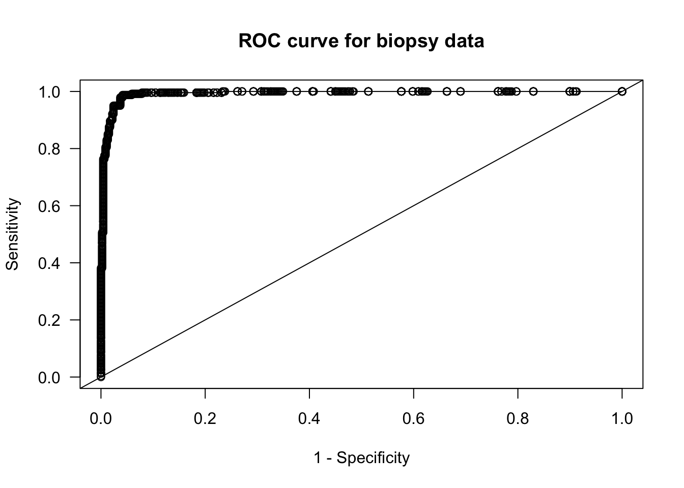

---

• Let’s compare the logistic regression ROC curve with a worthless risk score where we generate risk scores randomly from a uniform distribution.

rr <- runif(nrow(biopsy))
sorted.rr <- c(1, sort(rr, decreasing=TRUE), 0) 
mm <- length(sorted.rr)
roc.random.y <- roc.random.x <- rep(0, mm)
for(k in 1:mm) {
   thresh.val <- sorted.rr[k]
   roc.random.y[k] <- Sensitivity(thresh.val, Y=biopsy$tumor.type, rr)
   roc.random.x[k] <- 1 - Specificity(thresh.val, Y=biopsy$tumor.type, rr)
}
plot(roc.random.x, roc.random.y, main="ROC curve for biopsy data", xlab="1 - Specificity",
     ylab="Sensitivity", las=1, col="red", type="n")
lines(roc.random.x, roc.random.y, type="s", col="red")
lines(roc.x, roc.y, type="s")
legend("bottomright", legend=c("logistic regression risk scores", "random risk scores"),
       col=c("black", "red"), lwd=2, bty='n')
abline(0, 1)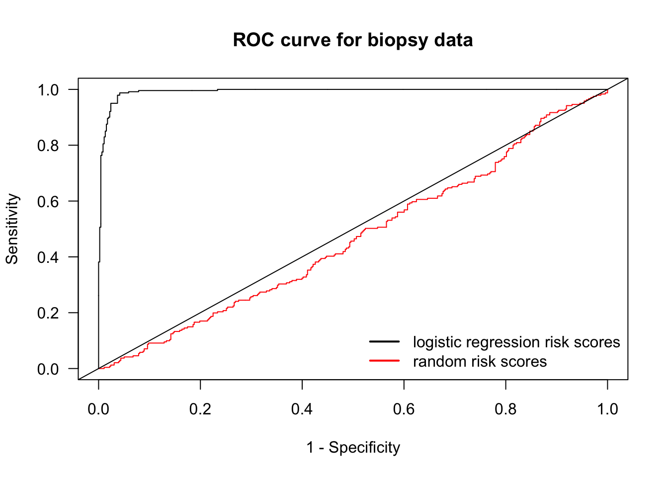

5.3 Area under the ROC curve

• The Area Under the ROC curve AUC is the area under the graph of the points $(x_{i}, y_{i})$, $i = 0, \ldots, n+1$.

• The AUC is given by $$\begin{equation} AUC = \sum_{i=0}^{n} y_{i}(x_{i+1} - x_{i}) \end{equation}$$

5.3.1 Rewriting the formula for the AUC

• Note that $$\begin{equation} y_{i} = \sum_{k=1}^{n} I\{ g(\mathbf{x}_{k}) \geq t_{(i)}\} I\{ Y_{k} = 1 \}\Big/\sum_{k=1}^{n} I\{ Y_{k} = 1\} = \frac{1}{n\hat{p}}\sum_{k=1}^{n} a_{ki}, \end{equation}$$ where $n\hat{p} = \sum_{k=1}^{n} I\{ Y_{k} = 1\}$ and $a_{ki} = I\{ g(\mathbf{x}_{k}) \geq t_{(i)}\} I\{ Y_{k} = 1 \}$.

• Because $t_{(i)} \geq t_{(i+1)}$: $$\begin{eqnarray} x_{i+1} - x_{i} &=& \sum_{k=1}^{n} \Big(I\{ g(\mathbf{x}_{k}) \geq t_{(i+1)}, Y_{k} = 0 \} - I\{ g(\mathbf{x}_{k}) \geq t_{(i)}, Y_{k} = 0 \}\Big)\Big/\sum_{k=1}^{n} I\{ Y_{k} = 0\} \nonumber \\ &=& \frac{1}{n(1 - \hat{p})}\sum_{k=1}^{n} I\{g(\mathbf{x}_{k}) < t_{(i)}\} I\{ g(\mathbf{x}_{k}) \geq t_{(i+1)}\} I\{Y_{k} = 0 \} \\ &=& \frac{1}{n(1 - \hat{p})}\sum_{k=1}^{n} I\{ g(\mathbf{x}_{k}) = t_{(i+1)}\} I\{Y_{k} = 0 \} \nonumber \\ &=& \frac{1}{n(1 - \hat{p})}\sum_{k=1}^{n} b_{ki} \end{eqnarray}$$ where $n(1 - \hat{p}) = \sum_{k=1}^{n} I\{ Y_{k} = 0\}$ and $b_{ki} = I\{ g(\mathbf{x}_{k}) = t_{(i+1)}\} I\{Y_{k} = 0 \}$.

---

• So, we can express the AUC as: $$\begin{eqnarray} AUC &=& \frac{1}{n^{2}\hat{p}(1 - \hat{p})}\sum_{i=0}^{n} \sum_{k=0}^{n} a_{ki} \sum_{k=0}^{n} b_{ki} = \frac{1}{n^{2}\hat{p}(1 - \hat{p})} \sum_{k=0}^{n} \sum_{j=0}^{n}\sum_{i=0}^{n} a_{ki} b_{ji} \\ &=& \frac{1}{n^{2}\hat{p}(1 - \hat{p})} \sum_{k=0}^{n} \sum_{j=0}^{n} I\{ Y_{k} = 1 \} I\{Y_{j} = 0 \} \sum_{i=0}^{n} I\{ g(\mathbf{x}_{k}) \geq t_{(i)}\}I\{ g(\mathbf{x}_{j}) = t_{(i+1)}\} \tag{5.1} \end{eqnarray}$$

• Note now that because the $t_{(i)}$ are the ordered values of the $g(\mathbf{x}_{h})$ $$\begin{equation} \sum_{i=0}^{n} I\{ g(\mathbf{x}_{k}) \geq t_{(i)}\}I\{ g(\mathbf{x}_{j}) = t_{(i+1)}\} = I\{ g(\mathbf{x}_{k}) \geq t_{(j^{*} - 1)}\} = I\{ g(\mathbf{x}_{k}) > t_{(j^{*})}\}, \end{equation}$$ where $j^{*}$ is the index such that $t_{(j^{*})} = g(\mathbf{x}_{j})$.

• Hence, $$\begin{equation} \sum_{i=0}^{n} I\{ g(\mathbf{x}_{k}) \geq t_{(i)}\}I\{ g(\mathbf{x}_{j}) = t_{(i+1)}\} = I\{ g(\mathbf{x}_{k}) > g(\mathbf{x}_{j}) \} \tag{5.2} \end{equation}$$

---

• Now, by plugging (5.2) into (5.1), we can finally express the AUC as $$\begin{eqnarray} AUC &=& \frac{1}{n^{2}\hat{p}(1 - \hat{p})} \sum_{k=0}^{n} \sum_{j=0}^{n} I\{ g(\mathbf{x}_{k}) > g(\mathbf{x}_{j}) \}I\{ Y_{k} = 1 \} I\{Y_{j} = 0 \} \end{eqnarray}$$

5.3.2 Interpreting the AUC

• We can write the AUC as $$\begin{equation} \textrm{AUC} = S_{1}/S_{2} \end{equation}$$

• The sum $S_{2}$ counts the number of all discordant pairs of responses

  • The pair of outcomes $(Y_{k}, Y_{j})$ is discordant if $Y_{k} = 1$ and $Y_{j}=0$ or vice versa. $$\begin{equation} S_{2} = \sum_{i=1}^{n}I\{ Y_{i} = 0\}\sum_{i=1}^{n} I\{Y_{i} = 1\} = \sum_{j=1}^{n}\sum_{k=1}^{n} I\{ Y_{j} = 0\} I\{Y_{k} = 1\} \end{equation}$$

• Now, look at the sum $S_{1}$: $$\begin{eqnarray} S_{1} &=& \sum_{k=0}^{n} \sum_{j=0}^{n} I\{ g(\mathbf{x}_{k}) > g(\mathbf{x}_{j}) \}I\{ Y_{k} = 1 \} I\{Y_{j} = 0 \} \end{eqnarray}$$

• $S_{1}$ looks at all discordant pairs of responses and counts the number of pairs where the risk score ordering agrees with the ordering of the responses.

---

• To summarize: The AUC is the proportion of discordant outcome pairs where the risk score ordering for that pair agrees with the ordering of the outcomes

• An AUC of $0.5$ means that the risk score is performing about the same as a risk score generated at random.

• The AUC is often referred to as the concordance index, or c-index.

---

• Let’s compute the AUC for our logistic regression-based risk score for the biopsy data:

AUC.biopsy <- sum(roc.y[-length(roc.y)]*diff(roc.x))
round(AUC.biopsy, 4)

## [1] 0.9928

• This is a very high AUC: $0.9928$

5.3.3 Computing the AUC in R

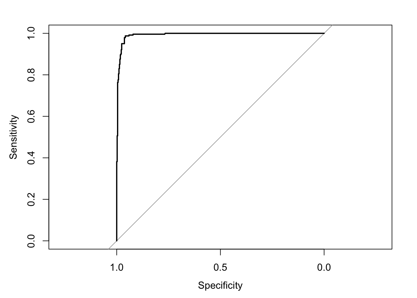
• You can compute the AUC in R without writing all your own functions by using the pROC package.

• With the pROC package, you start by inputting your binary outcomes and risk scores into the roc function in order to get an “roc object”.

library(pROC)
roc.biopsy <- roc(biopsy$tumor.type, risk.score)

• To find the AUC, you can then use auc(roc.biopsy)

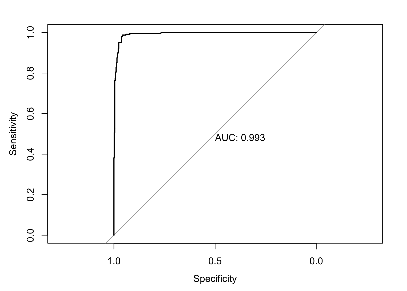
auc( roc.biopsy )

## Area under the curve: 0.9928

---

• You can plot the ROC curve by just plugging in the roc object into the plot function.

plot(roc.biopsy)

• To also print the AUC value, you can just add print.auc=TRUE

plot(roc.biopsy, print.auc=TRUE)

5.4 Calibration

• The AUC, or c-index is a measure of the statistical discrimination of the risk score.

• However, a high value of the AUC does not imply that the risk score is well-calibrated.

• Calibration refers to the agreement between observed frequency of the outcome and the fitted probabilities of those outcomes.

---

• For example, if we look at a group of individuals all of whom have a fitted probability of $0.2$, then we should expect that roughly $20\%$ of the outcomes should equal $1$ from this group.

• We can examine this graphically by looking at the observed proportion of successes vs. the fitted probabilities for several risk strata.

---

• Specifically, if we have risk score-cutoffs $r_{1}, \ldots, r_{G}$, the observed proportion of successes in the $k^{th}$ risk stratum is $$\begin{equation} O_{k} = \sum_{i=1}^{n} Y_{i}I\{ r_{k-1} < g(\mathbf{x}_{i}) \leq r_{k} \} \Big/\sum_{i=1}^{n} I\{ r_{k-1} < g(\mathbf{x}_{i}) \leq r_{k} \} \end{equation}$$

• The expected proportion of successes in the $k^{th}$ risk stratum is $$\begin{equation} P_{k} = \sum_{i=1}^{n} g(\mathbf{x}_{i})I\{ r_{k-1} < g(\mathbf{x}_{i}) \leq r_{k} \} \Big/\sum_{i=1}^{n} I\{ r_{k-1} < g(\mathbf{x}_{i}) \leq r_{k} \} \end{equation}$$

• If $g(\mathbf{x}_{i})$ is well-calibrated, $O_{k}$ and $P_{k}$ should be fairly similar for each $k$.

---

• Let’s make a calibration plot for the biopsy data.

• First, let’s make 10 risk strata using the quantiles of our logistic regression-based risk score.

rr <- c(0, quantile(risk.score, prob=seq(0.1, 0.9, by=0.1)), 1)
rr

##                     10%         20%         30%         40%         50% 
## 0.000000000 0.001505966 0.002756161 0.005385182 0.010154320 0.019231612 
##         60%         70%         80%         90%             
## 0.074574998 0.841857858 0.989561027 0.999471042 1.000000000

• Now, compute observed and expected frequencies for each of the risk strata and plot the result:

observed.freq <- pred.freq <- rep(0, 10)
for(k in 2:11) {
   ind <- risk.score <= rr[k] & risk.score > rr[k-1] # stratum indicators
   observed.freq[k] <- sum(biopsy$tumor.type[ind])/sum(ind)
   pred.freq[k] <- sum(risk.score[ind])/sum(ind)
}
plot(observed.freq, pred.freq, xlab="Observed Frequency",
     ylab = "Predicted Frequency",
     las=1, main="Calibration plot for biopsy data")
lines(observed.freq, pred.freq)
abline(0, 1, lty=2)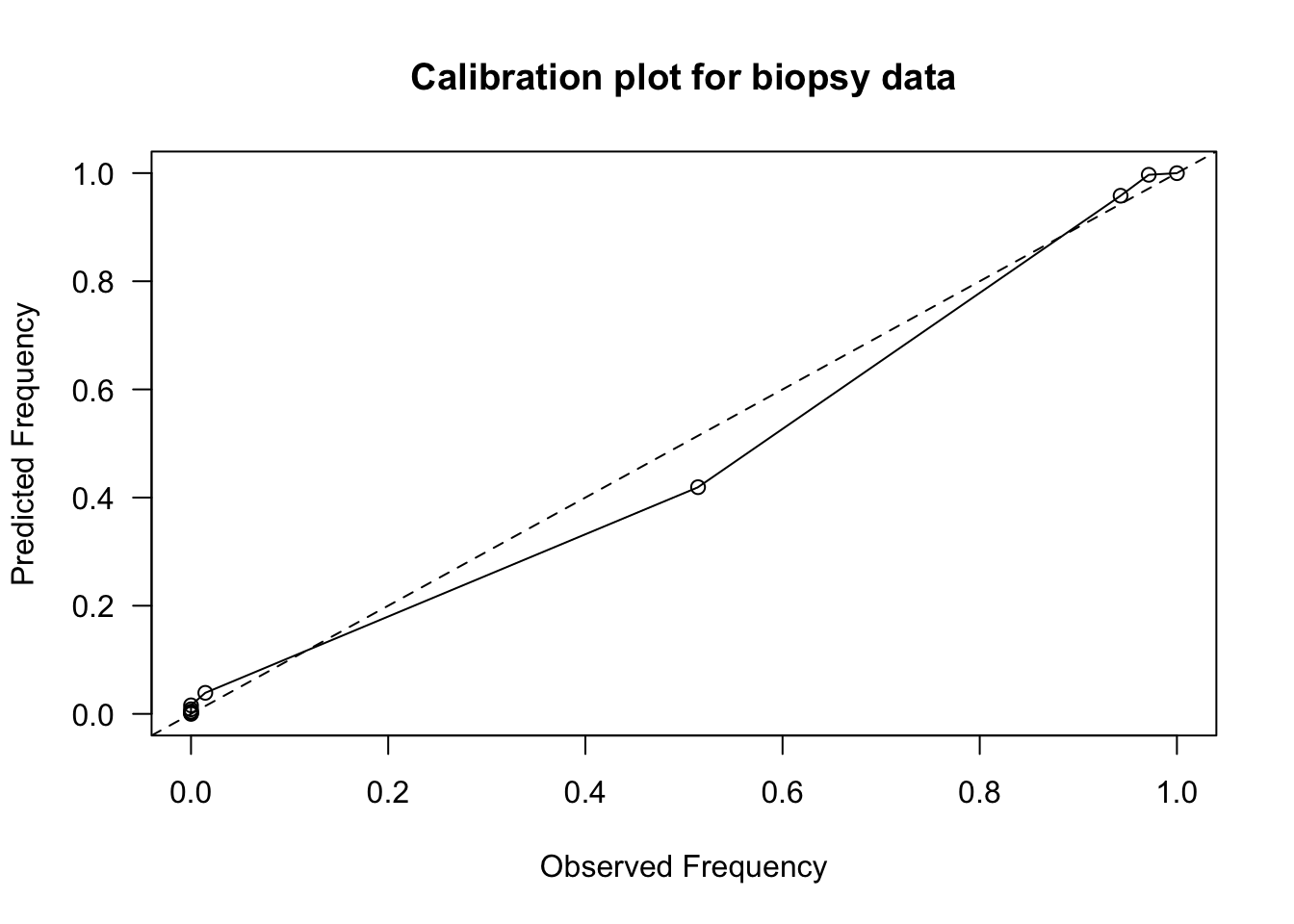

---

• Most of the risk scores are more concentrated near zero, but this calibration plot shows fairly good calibration.
  • Expected vs. Observed frequencies are mostly close to the $y = x$ straight line.
• Sometimes an estimated intercept and slope from a regression of expected vs. observed frequencies is reported.
  • We should expect that the intercept should be close to $0$ and the slope should be close to $1$ for a well-calibrated risk score.

lm(pred.freq ~ observed.freq)

## 
## Call:
## lm(formula = pred.freq ~ observed.freq)
## 
## Coefficients:
##   (Intercept)  observed.freq  
##      0.001759       0.994948

• The Hosmer–Lemeshow test is a more formal test that compares these types of observed vs. expected frequencies.

5.5 Longitudinal Data and Risk Score Validation

• When you have longitudinal responses $Y_{ij}$, sensitivity, specificity, and the AUC/c-index will depend on what exactly you are trying to predict.

• If you are trying to predict $Y_{ij} = 1$ vs. $Y_{ij} = 0$ for each $j$, sensitivity and specificity will be defined by $$\begin{equation} P\{ g(\mathbf{x}_{ij}) \geq t|Y_{ij} = 1\} \qquad \textrm{ and } \qquad P\{ g(\mathbf{x}_{ij}) < t|Y_{ij} = 0\} \end{equation}$$

• Here, $g(\mathbf{x}_{ij})$ would be a risk score based on covariate information up to and including time $t_{ij}$ and could include responses before time $t_{ij}$.

• In this case, the AUC would be calculated in the same way as the non-longitudinal case - you would just sum over all responses and risk scores across all individuals and time points.

---

• In other cases, you may want to predict a single outcome $\tilde{Y}_{i}$ even though the covariates are collected longitudinally over additional time points.

• For example, $\tilde{Y}_{i}$ might be an indicator of whether or not a patient is hypertensive over a particular time window.

• In this case, you might compute a single risk score $\hat{g}_{i}$ for each individual.

  • For example, $\hat{g}_{i} = \frac{1}{n_{i}}\sum_{j=1}^{n_{i}} g(\mathbf{x}_{ij})$.

  • For example, $\hat{g}_{i} = \textrm{median} \{ g(\mathbf{x}_{i1}), \ldots, g(\mathbf{x}_{in_{i}}) \}$.

  • For example, $\hat{g}_{i} = \max\{ g(\mathbf{x}_{i1}), \ldots, g(\mathbf{x}_{in_{i}}) \}$.

---

• To “validate” a risk score, you generally want to look at out-of-sample performance of the risk score.

• For example, you might build your risk model using data from individuals enrolled within a specific six-month time window and look at the AUC statistic for outcomes for individuals who enrolled in a different time window.

• Looking at the out-of-sample performance over a different time window or using data from a different source is often a good way of justifying the robustness/generalizability of a particular risk model.

---