Chapter 3 Nonparametric Regression with Longitudinal Data
3.1 Notation
For longitudinal data, we will again use the following notation:
Individual \(i\) has observations for both the outcome and the covariates at times \(t_{i1}, \ldots, t_{in_{i}}\)
\(Y_{ij}\) is the outcome for individual \(i\) at time \(t_{ij}\).
\(\mathbf{x}_{ij}\) is the vector of covariates at time \(t_{ij}\).
The \(i^{th}\) individual has \(n_{i}\) observations: \(Y_{i1}, \ldots, Y_{in_{i}}\).
There will be \(m\) individuals in the study (so \(1 \leq i \leq m\)).
A general regression model relating \(Y_{ij}\) and \(\mathbf{x}_{ij}\) is the following: \[\begin{equation} Y_{ij} = \mu( \mathbf{x}_{ij} ) + \varepsilon_{ij} \nonumber \end{equation}\]
Here, \(\mu(\mathbf{x}_{ij}) = E(Y_{ij}| \mathbf{x}_{ij})\) is the “mean function”.
In nonparametric approaches to estimating \(\mu(\cdot)\), we will try to estimate \(\mu(\mathbf{x})\) without making any strong assumptions about the form of \(\mu( \mathbf{x} )\).
Basically, in a nonparametric approach, there is not a fixed set of parameters describing the mean function that does not change as the sample size grows.
3.2 Kernel Smoothing
3.2.1 Description of Kernel Regression
With kernel regression, we estimate the mean function \(\mu(\mathbf{x})\) at \(\mathbf{x}\) by taking a weighted “local average” of the \(Y_{ij}\) around \(\mathbf{x}\).
Specifically, the kernel regression estimate of \(\mu(\cdot)\) at a point \(\mathbf{x}\) can be expressed as \[\begin{equation} \hat{\mu}( \mathbf{x} ) = \sum_{i=1}^{m}\sum_{j=1}^{n_{i}} w_{ij}(\mathbf{x})Y_{ij} \end{equation}\]
The “weights” at the point \(\mathbf{x}\) are given by \[\begin{equation} w_{ij}(\mathbf{x}) = \frac{ K\Big( \frac{\mathbf{x} - \mathbf{x}_{ij}}{ h_{n} }\Big) }{ \sum_{i=1}^{m}\sum_{j=1}^{n_{i}} K\Big( \frac{\mathbf{x} - \mathbf{x}_{ij}}{ h_{n} }\Big) } \tag{3.1} \end{equation}\]
When using the weights (3.1), \(\hat{\mu}(\mathbf{x})\) is known as the Nadaraya-Watson esitmator.
The function \(K(\cdot)\) in (3.1) is referred to as the “kernel function”.
The kernel function \(K(\cdot)\) is:
- A smooth nonnegative function
- Symmetric around \(0\)
- Has a mode at \(0\) and decays the further you go away from \(0\)
A common choice of \(K(\cdot)\) is the Gaussian kernel \[\begin{equation} K(\mathbf{u}) = \exp\Big\{ - \frac{||\mathbf{u}||^{2}}{2} \Big\} \end{equation}\]
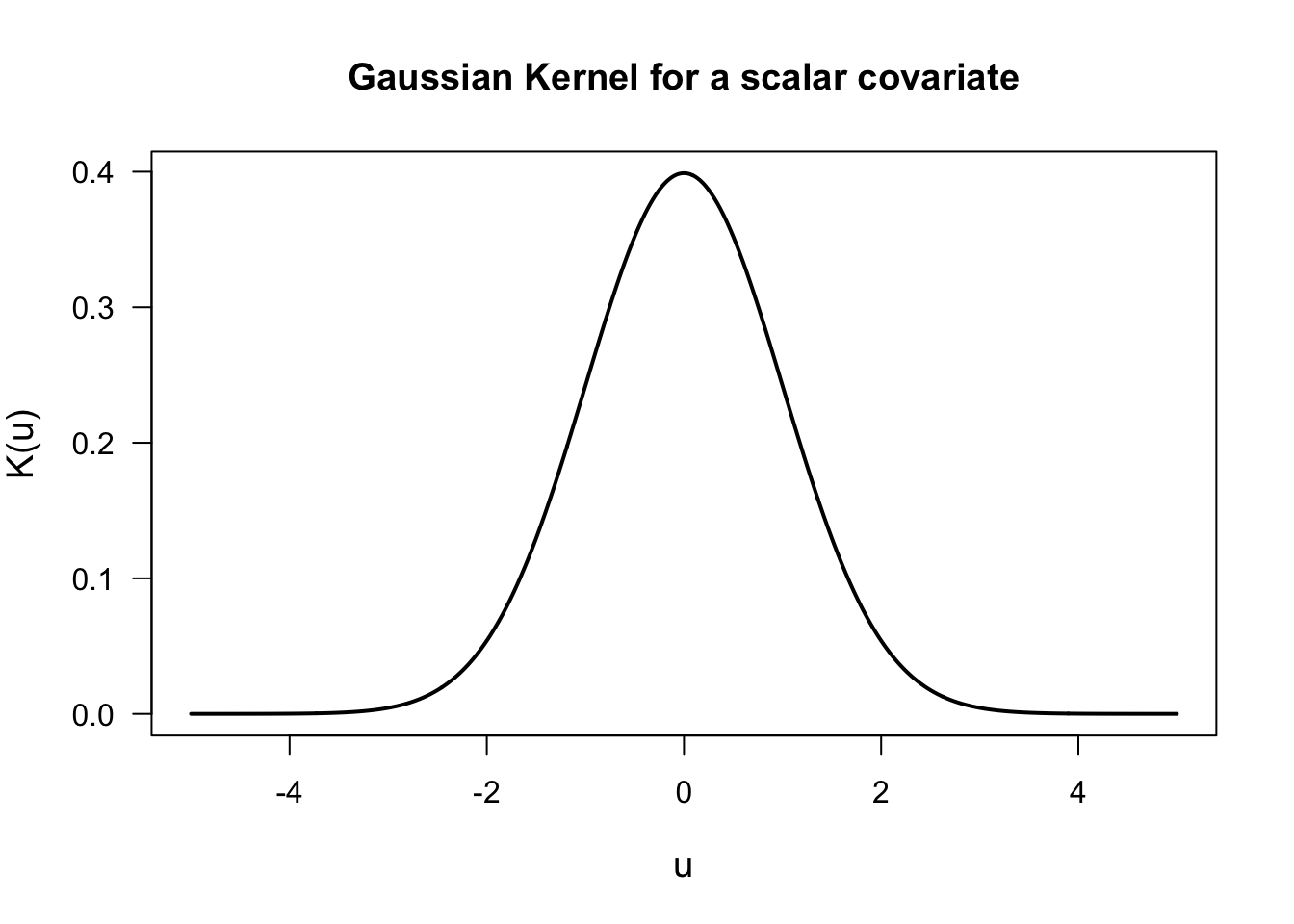
Observations where \(\mathbf{x}_{ij}\) is “close” to \(\mathbf{x}\) will be given a larger weight \(w_{ij}(\mathbf{x})\) because \(||\mathbf{x} - \mathbf{x}_{ij}||^{2}\) will be small.
Similarly, observations where \(\mathbf{x}_{ij}\) is “far away” from \(\mathbf{x}\) will be given a smaller weight \(w_{ij}(\mathbf{x})\) because \(||\mathbf{x} - \mathbf{x}_{ij}||^{2}\) will be small.
The term \(h_{n} > 0\) is referred to as the bandwidth.
The bandwidth determines how many observations have a strong impact on the value of \(\hat{\mu}( \mathbf{x} )\).
If the bandwidth \(h_{n}\) is small, observations close to \(\mathbf{x}\) will largely determine the value of \(\hat{\mu}(\mathbf{x})\).
If the bandwidth \(h_{n}\) is large, the value of \(\hat{\mu}(\mathbf{x})\) will be more heavily influenced by a larger number of observations.
Kernel regression estimates with a smaller bandwidth will be more “wiggly” and non-smooth.
Kernel regression estimates with a larger bandwidth will be more smooth.
3.2.2 Kernel Regression in the sleepstudy data
Again, let’s look at the sleepstudy data from the lme4 package.
The sleepstudy data had 18 participants with reaction time measured across 10 days.
## Loading required package: Matrix## Reaction Days Subject
## 1 249.5600 0 308
## 2 258.7047 1 308
## 3 250.8006 2 308
## 4 321.4398 3 308
## 5 356.8519 4 308
## 6 414.6901 5 308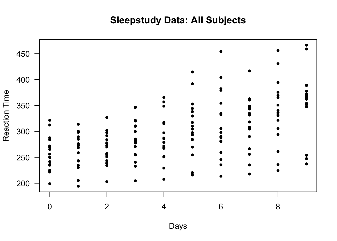
We can estimate the marginal mean function for the sleepstudy data by using a GEE.
We will assume that reaction time is a linear function of time on study:
- That is, we will assume that \(\mu(t) = \beta_{0} + \beta_{1} t\).
library(geepack)
## Use AR(1) correlation structure
sleep.gee <- geeglm(Reaction ~ Days, data=sleepstudy, id=Subject, corstr="ar1") - To get the value of the estimated regression function, we can use the first \(10\) fitted values (because the fitted values for each subject are the same as the overall mean function)
## Estimated mean function at each time point
gee.regfn <- sleep.gee$fitted.values[1:10,1]

### Now plot the estimated mean function
plot(sleepstudy$Days, sleepstudy$Reaction, las=1, ylab="Reaction Time", xlab="Days",
     main="Sleepstudy: GEE estimate of Mean Function", type="n")
points(sleepstudy$Days, sleepstudy$Reaction, pch=16, cex=0.8)
lines(0:9, gee.regfn, lwd=2, col="red")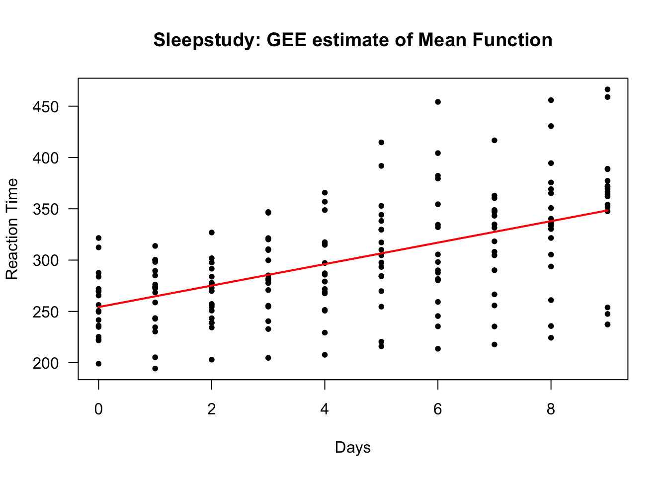
To find a kernel regression estimate of the mean function, you can use the ksmooth function in R.
One thing to note is that ksmooth only works for a scalar covariate.
Using a bandwidth of \(0.5\) and a Gaussian kernel, we can find the kernel regression estimate of the mean function with the following R code:
This will return a list with an “x vector” and a “y vector”.
The
xvector will be the vector of points at which the regression function is estimated. Theyvector will be a vector containing the estimated values of the regression function.
- Let’s plot the estimated mean function to see what it looks like:
plot(sleepstudy$Days, sleepstudy$Reaction, las=1, ylab="Reaction Time", xlab="Days",
     main="Sleepstudy: Kernel Regression with Bandwidth = 0.5", type="n")
points(sleepstudy$Days, sleepstudy$Reaction, pch=16, cex=0.8)
lines(sleep.kernel$x, sleep.kernel$y, lwd=2, col="red")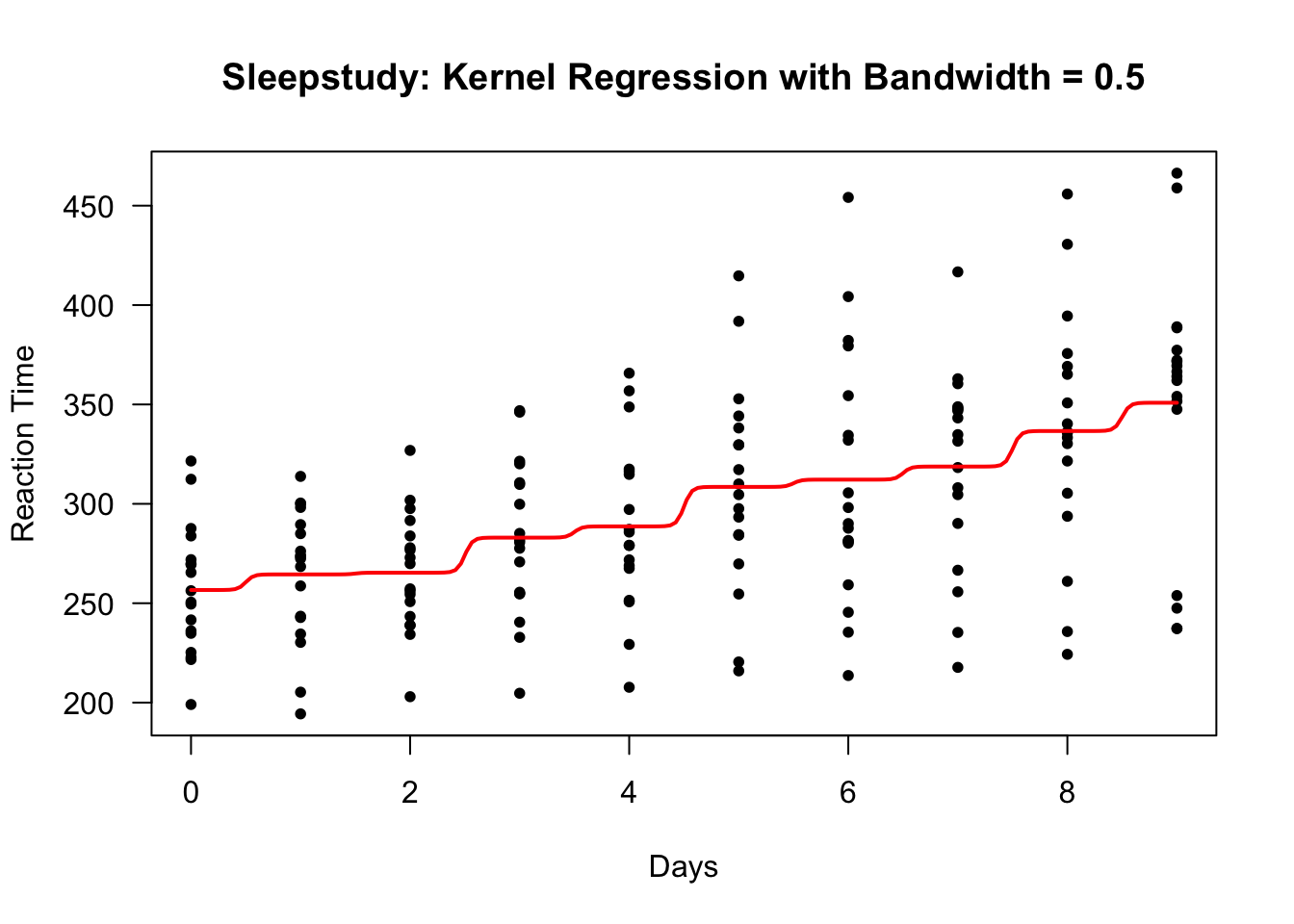
This bandwidth looks too small. There are clear “near jumps” in between some of the days.
We can try a bandwidth of \(1\) to see if we can smooth this out a bit.
sleep.kernel.bw1 <- ksmooth(sleepstudy$Days, sleepstudy$Reaction, kernel="normal",
                        bandwidth = 1)

plot(sleepstudy$Days, sleepstudy$Reaction, las=1, ylab="Reaction Time", xlab="Days",
     main="Sleepstudy: Kernel Regression with Bandwidth = 1", type="n")
points(sleepstudy$Days, sleepstudy$Reaction, pch=16, cex=0.8)
lines(sleep.kernel.bw1$x, sleep.kernel.bw1$y, lwd=2, col="red")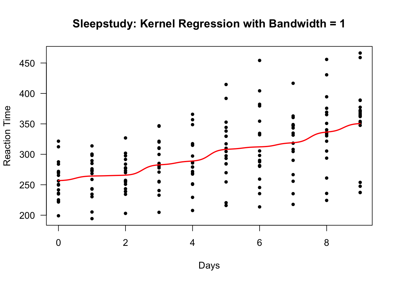
3.2.3 Bandwidth Selection
The bandwidth can be chosen to get a level of smoothness that looks good visually.
For example, when observations are only collected daily like in the sleepstudy you will probably want to choose a bandwidth so that the estimated mean function does not have obvious bumps in between days.
To choose the bandwidth \(h_{n} > 0\) using a formal criterion, a common approach is to use leave-one-out cross-validation.
In the context of longitudinal data, it is usually suggested that you leave one subject out at a time rather than one observation at a time (Rice and Silverman (1991)).
The reason for this is that the subject-level leave-one-out cross-validation score is a good estimate of the mean-squared prediction error of regardless of what the correlation structure is for the within-subject outcomes.
This is not the case when using observation-level leave-one-out cross-validation.
The subject-level leave-one-out cross-validation score for a given bandwidth choice is defined as \[\begin{equation} \textrm{LOOCV}(h_{n}) = \sum_{i=1}^{n}\sum_{j=1}^{m_{i}} \{ Y_{ij} - \hat{\mu}_{h_{n}}^{(-i)}(\mathbf{x}_{ij}) \}^{2} \end{equation}\]
Here, \(\hat{\mu}_{h_{n}}^{(-i)}(\mathbf{x}_{ij})\) is the mean function estimate when using bandwidth \(h_{n}\) and when ignoring the data from subject \(i\).
3.2.4 Another Example: The Bone Data
As another example, we can use the “bone” dataset.
This is a longitudinal dataset with typically 2 or 3 observations per individual.
The outcome variable of interest is the relative spinal bone mineral density.
This is actual the difference in mineral density taken on two consecutive visits divided by the average mineral density on those visits.
bonedat <- read.table("https://web.stanford.edu/~hastie/ElemStatLearn/datasets/bone.data",
                      header=TRUE)
head(bonedat)
## idnum age gender spnbmd
## 1 1 11.70 male 0.018080670
## 2 1 12.70 male 0.060109290
## 3 1 13.75 male 0.005857545
## 4 2 13.25 male 0.010263930
## 5 2 14.30 male 0.210526300
## 6 2 15.30 male 0.040843210- For this data, the interest would be to model the mean function for bone mineral
density (the variable
spnbmd) as a function ofage

- We can compute the leave-one-out cross-validation score for the bone data for different values of \(h_{n}\) (here \(0.1 \leq h_{n} \leq 1\)) with the following code:
nh <- 200
hh <- seq(.1, 1, length.out=nh)
LOOCV <- rep(0, nh)
subj.list <- unique(bonedat$idnum)
nsubj <- length(subj.list)
for(k in 1:nh) {
    ss <- 0
    for(i in 1:nsubj) {
        ind <- bonedat$idnum==subj.list[i]
        yy <- bonedat$spnbmd[-ind]
        xx <- bonedat$age[-ind]
        tmp <- ksmooth(xx, yy, kernel="normal", bandwidth = hh[k],
                       x.points=bonedat$age[ind])
        mu.hat <- tmp$y
        ss <- ss + sum((bonedat$spnbmd[ind] - mu.hat)^2)
    }
    LOOCV[k] <- ss
}
hh[which.min(LOOCV)] ## best seems to be 0.1
## [1] 0.1- In this case, the best bandwidth was \(0.1\) according to the subject-level leave-one-out cross-validation criterion.
- The kernel regression estimate of the mean function with the bandwidth of \(0.1\) is plotted below:
bone.kernel <- ksmooth(bonedat$age, bonedat$spnbmd, kernel="normal",
                        bandwidth = 0.1, x.points=seq(9.4, 25, length.out=100))

plot(bonedat$age, bonedat$spnbmd, las=1, ylab="spnbmd", xlab="age",
     main="Bone Data: Kernel Regression with Bandwidth = 0.1", type="n")
points(bonedat$age, bonedat$spnbmd, pch=16, cex=0.8)
lines(bone.kernel$x, bone.kernel$y, lwd=2, col="red")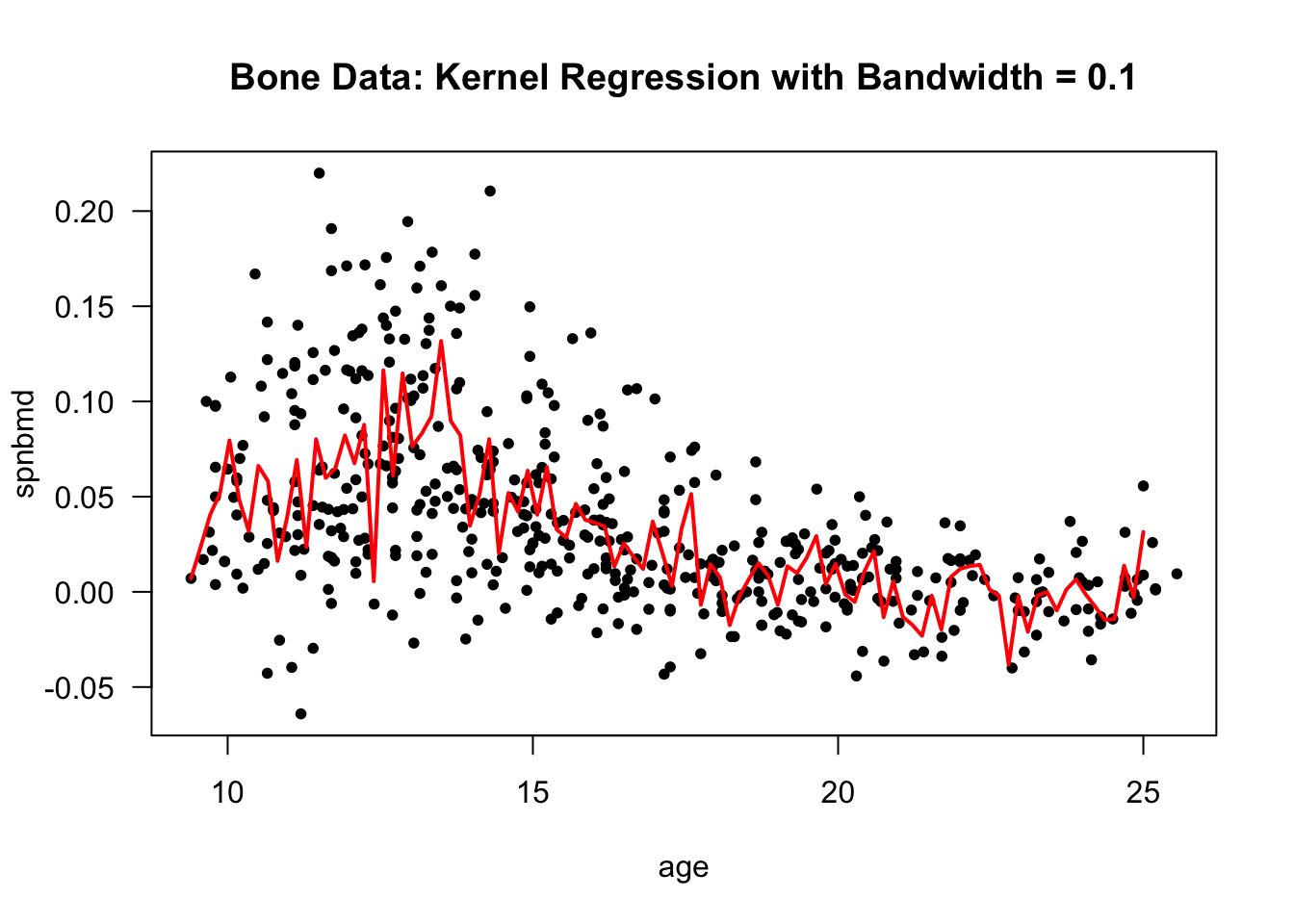
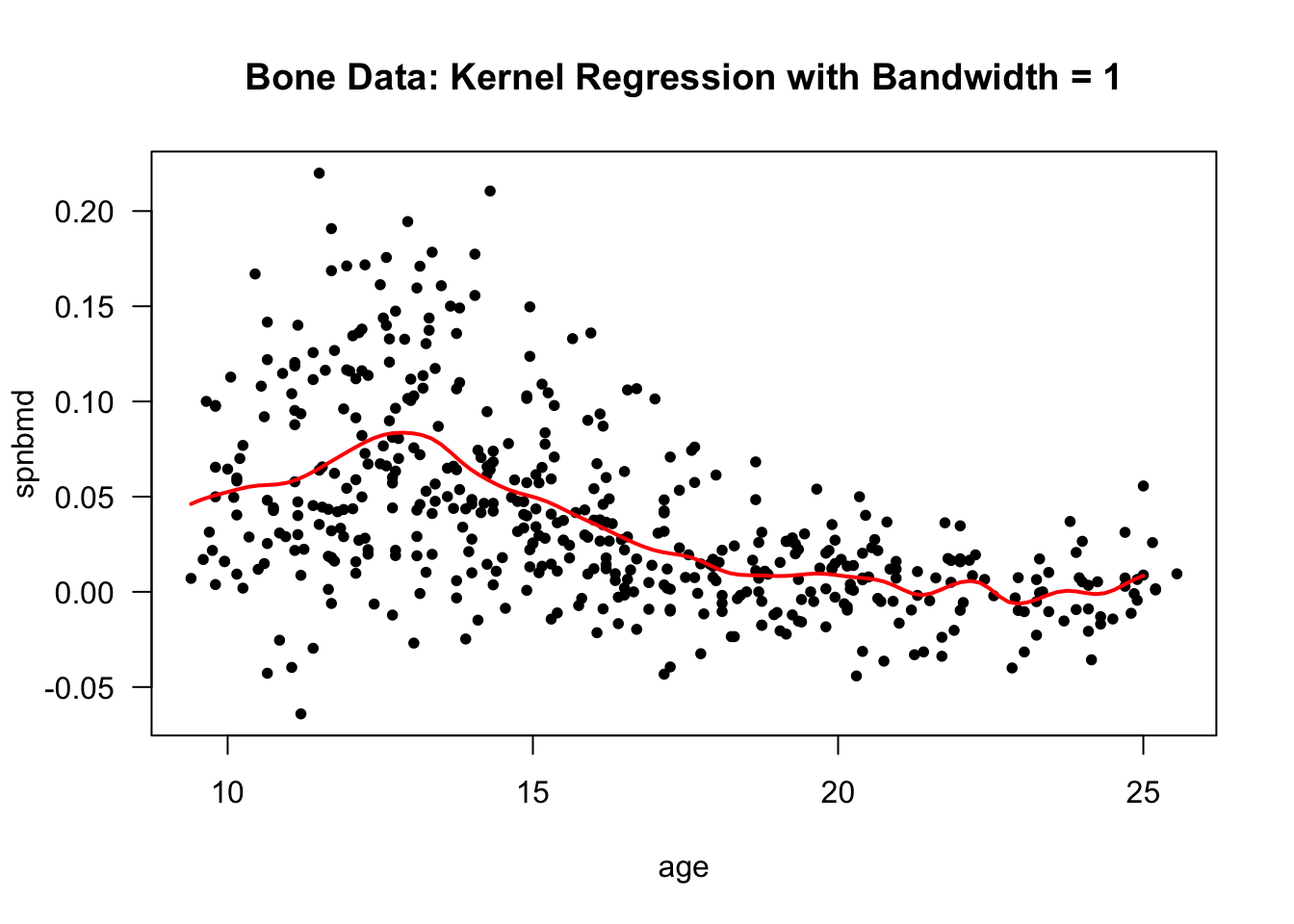
- Using a bandwidth of \(1\) gives a smoother mean function estimate.
The performance of kernel regression methods can degrade quickly as we move to higher dimensions. The convergence rate of the estimated regression function to the true regression function slows substantially as we the dimension of the covariates \(\mathbf{x}_{ij}\).
“Curse of dimensionality” - need very large datasets to have a sufficient number of observations near a given point \(\mathbf{x}\).
Another approach when using multiple covariates is to use generalized additive models.
With generalized additive models, the mean function is expressed as the sum of several univariate nonparametric functions: \[\begin{equation} \mu(\mathbf{x}) = \beta_{0} + \mu(x_{1}) + \mu(x_{2}) + \ldots + \mu(x_{p}) \end{equation}\]
3.3 Regression Splines
3.3.1 Overview
Using regression splines is a common nonparametric approach for estimating a mean function.
The most common type of spline used in the context of nonparametric regression is the cubic spline.
Definition: A cubic spline with knots \(u_{1} < u_{2} < \ldots < u_{q}\) is a function \(f(x)\) such that
- \(f(x)\) is a cubic function over each of the intervals \((-\infty, u_{1}], [u_{1}, u_{2}], \ldots, [u_{q-1}, u_{q}], [u_{q}, \infty)\).
- \(f(x)\), \(f'(x)\), and \(f''(x)\) are all continuous functions.
A commonly used set of basis functions for the set of cubic splines with knots \(u_{1} < u_{2} < \ldots < u_{q}\) is the B-spline basis functions.
This means that if \(\varphi_{1, B}(x), \ldots, \varphi_{q+4, B}(x)\) are the B-spline basis functions for the set of cubic splines with knots \(u_{1} < u_{2} < \ldots < u_{q}\), we can represent any cubic spline estimate of the mean function as \[\begin{equation} \hat{\mu}(x) = \sum_{j=1}^{q+4} \hat{\beta}_{j}\varphi_{j, B}(x) \end{equation}\]
The nice thing about using regression splines is that they can estimated in the same way as in a “typical” regression setting.
For regression splines, the columns of the design matrix contain the values of \(\varphi_{j,B}(x_{i})\).
3.3.2 Regression Splines with Longitudinal Data in R
- Regression splines can be fitted in R by using the
splinespackage
- The
bsfunction insplinesgenerates the B-spline “design” matrix
x- vector of covariates values. This can also just be the name of a variable whenbsis used inside a function such asgeeglm.df- the “degrees of freedom”. For a cubic spline this is actually \(q + 3\) rather than \(q + 4\). If you just enterdf, thebsfunction will pick the knots for you.knots- the vector of knots. If you don’t want to pick the knots, you can just enter a number for thedf.degree- the degree of the piecewise polynomial. Typically,degree=3which would be a cubic spline.
You can directly use regression splines within the “GEE framework”.
In this case, you can model the marginal mean (or part of the marginal mean function) with a spline.
Here, we are assuming that \(E(Y_{ij}|t_{ij}) = f_{0}(t_{ij})\) with:
- \(Y_{ij}\) is the
spnbmdvalue of individual \(i\) at age \(t_{ij}\). - \(t_{ij}\) is the \(j^{th}\) age value of individual \(i\)
- The function \(f_{0}(t)\) will be estimated with a spline.
- \(Y_{ij}\) is the
To fit this with an AR1 correlation structure, you would use the following code:
- The argument
df = 6means that the number of columns in the design matrix is 7 (due to the intercept), and the number of knots is is determined by the equation \(q + 4 = 7\) (so \(q = 3\)).- You can actually explicity define the set of knots using the
knotsargument if you would like.
- You can actually explicity define the set of knots using the
- We can look at the estimates of the regression coefficients by using
summary.
##
## Call:
## geeglm(formula = spnbmd ~ bs(age, df = 6), data = bonedat, id = idnum,
##     corstr = "ar1")
##
##  Coefficients:
##                  Estimate  Std.err   Wald Pr(>|W|)
## (Intercept)       0.05124  0.01580 10.518  0.00118 **
## bs(age, df = 6)1 -0.01790  0.03214  0.310  0.57751
## bs(age, df = 6)2  0.06437  0.01647 15.281 9.27e-05 ***
## bs(age, df = 6)3 -0.03130  0.02028  2.383  0.12263
## bs(age, df = 6)4 -0.04220  0.01668  6.398  0.01142 *
## bs(age, df = 6)5 -0.06118  0.01951  9.837  0.00171 **
## bs(age, df = 6)6 -0.03974  0.01687  5.549  0.01849 *
## ---
## Signif. codes:  0 '***' 0.001 '**' 0.01 '*' 0.05 '.' 0.1 ' ' 1
##
## Correlation structure = ar1
## Estimated Scale Parameters:
##
##             Estimate  Std.err
## (Intercept) 0.001623 0.000135
##   Link = identity
##
## Estimated Correlation Parameters:
##       Estimate Std.err
## alpha   0.2872 0.06967
## Number of clusters: 261 Maximum cluster size: 3- There’s not really any interpretation to the individual regression coefficients estimates in a spline model
- You would typically be more interested in plotting the fitted values as a function of age.
- The
gee.bone0object has a component called “fitted values” which contains the values of \(\hat{f}_{0}(t_{ij})\) for each \(t_{ij}\).
## [1] 11.70 12.70 13.75 13.25 14.30## [1] 0.07000 0.08114 0.07288 0.07918 0.06279- To plot the estimated mean function, we can just draw lines through the fitted values:
plot(bonedat$age, bonedat$spnbmd, xlab="age", ylab="spnbmd",
     main="Regression Spline Estimate for Bone Data", las=1)
lines(bonedat$age[order(bonedat$age)],
      gee.bone0$fitted.values[order(bonedat$age)], lwd=2) ## plot spline estimate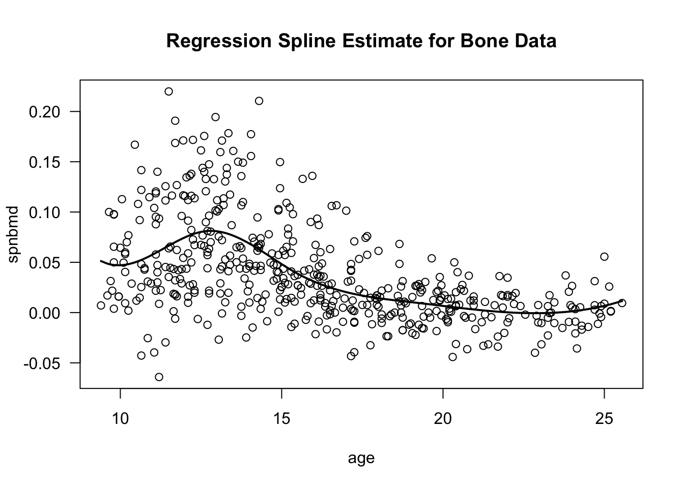
3.3.3 Looking at a Continuous and a Binary Covariate
For example, with the bone data, suppose we want to fit separate curves for the male and female groups.
We could express the mean function \(\mu(\cdot)\) as \[\begin{equation} \mu(t_{ij}) = f_{0}(t_{ij}) + A_{ij}f_{1}(t_{ij}) \tag{3.2} \end{equation}\]
\(f_{0}(\cdot)\) and \(f_{1}(\cdot)\) would be modeled with regression splines.
\(t_{ij}\) is the value of age for observation \((i,j)\)
\(A_{ij} = 1\) if the \((i,j)\) observation corresponds to a male individual and \(A_{ij} = 0\) if the \((i,j)\) observation corresponds to a female individual.
- To fit model (3.2) using the
geepackpackage, you can use the following code
library(splines)
gee.bone01 <- geeglm(spnbmd ~ bs(age, df=6) + gender*bs(age,df=6), id=idnum, data=bonedat,
corstr="ar1")- We can plot the estimated mean functions by first extracting the fitted values for both the male and female groups:
male.fitted <- gee.bone01$fitted.values[bonedat$gender=="male"]
male.age <- bonedat$age[bonedat$gender=="male"]
female.fitted <- gee.bone01$fitted.values[bonedat$gender=="female"]
female.age <- bonedat$age[bonedat$gender=="female"]- Now, plot the fitted curves for both groups
plot(bonedat$age, bonedat$spnbmd, lwd=1, xlab="age", ylab="spnbmd",
     main="Regression Splines for the Bone Data", las=1)
points(bonedat$age[bonedat$gender=="male"], bonedat$spnbmd[bonedat$gender=="male"],
       cex=0.8)
points(bonedat$age[bonedat$gender=="female"], bonedat$spnbmd[bonedat$gender=="female"],
       pch=16, cex=0.8)
lines(male.age[order(male.age)], male.fitted[order(male.age)], col="red", lwd=2)
lines(female.age[order(female.age)], female.fitted[order(female.age)], col="blue",
      lwd=2)
legend("topright", legend=c("Male", "Female"), col=c("red", "blue"), lwd=3, bty='n')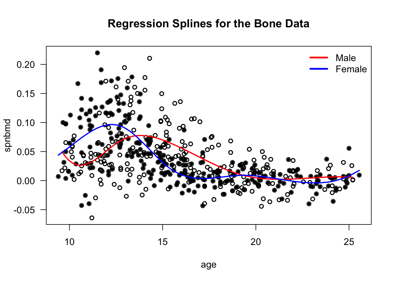
We could also fit a model where there is a simple “male” effect that does not change over time. \[\begin{equation} \mu(t_{ij}) = f_{0}(t_{ij}) + \beta_{1}A_{ij} \end{equation}\]
The mean function for male individuals would be \(f_{0}(t) + \beta_{1}\).
The mean function for females would be \(f_{0}(t)\).
This could be fit with the following code:
If we plot the estimated mean functions from
gee.bone1, it looks like the following:
I think the model \(\mu(t_{ij}) = f_{0}(t_{ij}) + \beta_{1}A_{ij}\) is just not a good one.
- Forcing the mean function to have this form hides the differences between males/females.
3.3.4 Model Comparison
We just fit the following three models \[\begin{eqnarray} \mu(t_{ij}) &=& f_{0}(t_{ij}) \\ \mu(t_{ij}) &=& f_{0}(t_{ij}) + \beta_{1}A_{ij} \\ \mu(t_{ij}) &=& f_{0}(t_{ij}) + A_{ij}f_{1}(t_{ij}) \end{eqnarray}\]
These model fits were saved as
gee.bone0,gee.bone1, andgee.bone01.
We can formally compare the models using the
anovamethod in RTo compare, \(\mu(t_{ij}) = f_{0}(t_{ij})\) vs. \(\mu(t_{ij}) = f_{0}(t_{ij}) + \beta_{1}A_{ij}\) do the following:
## Analysis of 'Wald statistic' Table
##
## Model 1 spnbmd ~ bs(age, df = 6) + gender
## Model 2 spnbmd ~ bs(age, df = 6)
##   Df    X2 P(>|Chi|)
## 1 1 0.164 0.69- This p-value is quite large (0.69). This is saying there is not strong evidence favoring
model \(\mu(t_{ij}) = f_{0}(t_{ij}) + \beta_{1}A_{ij}\) over the more simple model
\(\mu(t_{ij}) = f_{0}(t_{ij})\).
- In other words, a model with a single “male effect” is not better than a nonparametric model that does not take male/female into consideration.
- Now, let’s compare the models \(\mu(t_{ij}) = f_{0}(t_{ij})\) vs. \(\mu(t_{ij}) = f_{0}(t_{ij}) + A_{ij}f_{1}(t_{ij})\)
## Analysis of 'Wald statistic' Table
##
## Model 1 spnbmd ~ bs(age, df = 6) + gender * bs(age, df = 6)
## Model 2 spnbmd ~ bs(age, df = 6)
##   Df   X2 P(>|Chi|)
## 1  7 62.1   5.9e-11 ***
## ---
## Signif. codes:  0 '***' 0.001 '**' 0.01 '*' 0.05 '.' 0.1 ' ' 1
Here, we see a very small p-value.
This is strong evidence in favor of the model \(\mu(t_{ij}) = f_{0}(t_{ij}) + A_{ij}f_{1}(t_{ij})\) over the model \(\mu(t_{ij}) = f_{0}(t_{ij})\).
3.3.5 ACTG trial example
actg_trial <- read.csv("~/Library/Mobile Documents/com~apple~CloudDocs/Documents/HDS629/actg_trial.csv")- When you load the dataset into R, it should look like the following
##    SubjectID Treatment   Age Sex   Week   CD4
## 1          1         2 36.43   1  0.000 3.135
## 2          1         2 36.43   1  7.571 3.045
## 3          1         2 36.43   1 15.571 2.773
## 4          1         2 36.43   1 23.571 2.833
## 5          1         2 36.43   1 32.571 3.219
## 6          1         2 36.43   1 40.000 3.045
## 7          2         4 47.85   1  0.000 3.068
## 8          2         4 47.85   1  8.000 3.892
## 9          2         4 47.85   1 16.000 3.970
## 10         2         4 47.85   1 23.000 3.611
This longitudinal dataset has 5036 observations with the following 6 variables:
- SubjectID - subject identifier
Treatment - treatment received (4 possible treatments)
Age - age in years at baseline
Sex - 1=M, 0=F
Week - time in weeks from baseline
CD4 - this is the natural logarithm of the CD4 count + 1
Note that Treatment should be a factor variable
Let’s plot of CD4 vs. week for just individuals in Treatment 1. This plot includes a lowess smoothing line.
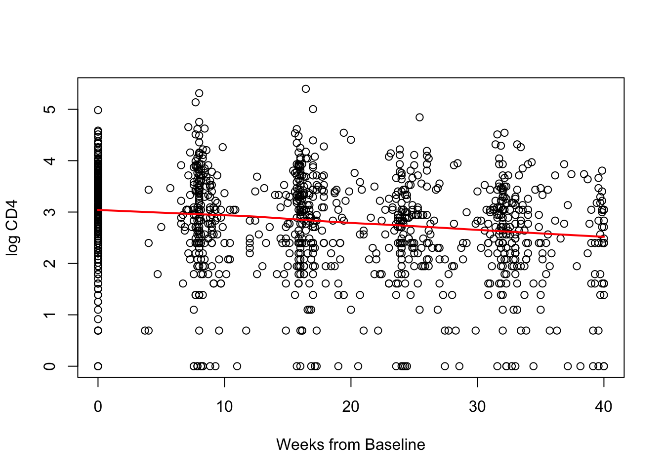
Not any clear evidence that change in CD4 over time is not linear in the treatment 1 group.
We can compare the following two models \[\begin{eqnarray} \mu(t_{ij}) &=& \beta_{0} + \beta_{1}t_{ij} \\ \mu(t_{ij}) &=& f_{0}(t_{ij}) \end{eqnarray}\] where \(f_{0}\) will be modeled with a spline function.
- We can fit these two models with
geeglmusing the following code:
actg_trt1_linear <- geeglm(CD4 ~ Week, id=SubjectID, data=Trt1Dat,
                           corstr="ar1")

actg_trt1_spline <- geeglm(CD4 ~ bs(Week, df=4), id=SubjectID, data=Trt1Dat,
corstr="ar1")- Now, do a formal comparison:
## Analysis of 'Wald statistic' Table
##
## Model 1 CD4 ~ bs(Week, df = 4)
## Model 2 CD4 ~ Week
##   Df    X2 P(>|Chi|)
## 1  3 0.975      0.81
No evidence to favor the nonparametric model over the linear model.
For this type of data where, the time point of observations fall into clear “groups”, another direct nonparametric approach is just to have an indicator for each one of the time groups (e.g., weeks 0 - 5, weeks 5-12, weeks 12-20, etc.)
Now, suppose we are interested in looking at differences in response to treatments in some way.
Consider the following 3 models (where \(A_{i}\) is treatment assigned at baseline): \[\begin{eqnarray} \mu(t_{ij}, a) &=& \beta_{0} + \beta_{1}t_{ij} \\ \mu(t_{ij}, a) &=& \beta_{0} + \beta_{1}t_{ij} + I(A_{i}=a, a \geq 2)\beta_{a} \\ \mu(t_{ij}, a) &=& \beta_{0} + \beta_{1}t_{ij} + I(A_{i}=a, a \geq 2)\beta_{a} + I(A_{i}=a, a \geq 2)\gamma_{a}t_{ij} \\ \end{eqnarray}\]
Now, the mean function depends on time and treatment
What is the interpretation of each of these models? Which model does not really make sense since this is a randomized trial?
actg_mod1 <- geeglm(CD4 ~ Week, id=SubjectID, data=actg_trial,
                           corstr="ar1")

actg_mod2 <- geeglm(CD4 ~ Week + Treatment, id=SubjectID, data=actg_trial,
                           corstr="ar1")

actg_mod3 <- geeglm(CD4 ~ Week*Treatment, id=SubjectID, data=actg_trial,
corstr="ar1")- Compare model 3 vs model 2
## Analysis of 'Wald statistic' Table
##
## Model 1 CD4 ~ Week * Treatment
## Model 2 CD4 ~ Week + Treatment
##   Df   X2 P(>|Chi|)
## 1  3 49.7   9.4e-11 ***
## ---
## Signif. codes: 0 '***' 0.001 '**' 0.01 '*' 0.05 '.' 0.1 ' ' 1- Compare model 2 vs model 1
## Analysis of 'Wald statistic' Table
##
## Model 1 CD4 ~ Week + Treatment
## Model 2 CD4 ~ Week
##   Df   X2 P(>|Chi|)
## 1  3 6.53     0.089 .
## ---
## Signif. codes:  0 '***' 0.001 '**' 0.01 '*' 0.05 '.' 0.1 ' ' 1
How would we fit the model \[\begin{equation} \mu(t_{ij}, a) = \beta_{0} + \beta_{1}t_{ij} + I(A_{i}=a, a \geq 2)\gamma_{a}t_{ij} \end{equation}\]
Use:
3.3.6 Treatment Comparisons for the ACTG trial
For data like that in
actg_trial, one is often interested in reporting measures which quantify the effect of different treatments.For treatment comparisons, it can be useful to thing about the “potential outcomes” of each individual.
The potential outcome \(Y_{ij}^{(a)}\) is the outcome for subject \(i\) at time \(t_{ij}\) if that subject had received treatment \(a\) (where \(a=1,2,3,4\)).
Note that we do not observed \(Y_{ij}^{(a)}\) for all four possible treatments.
We only observe \(Y_{ij}^{(a)}\) for the treatment that subject \(i\) received.
As a starting point for treatment comparisons, it is useful to first define what the “treatment effect” would be for subject \(i\) if we could observe all of subject i’s potential outcomes.
- We will define this unobserved treatment effect of treatment a vs. treatment b as \(Z_{i}^{ab}\).
For longitudinal data, the way to think about this treatment effect will depend somewhat on the context of the study.
One possible way to define \(Z_{i}^{ab}\) is to compare change in response over time: \[\begin{equation} Z_{i}^{ab} = (Y_{iJ}^{(a)} - Y_{i1}^{(a)}) - (Y_{iJ}^{(b)} - Y_{i1}^{(b)}) \end{equation}\]
Another reasonable way to define \(Z_{i}^{ab}\) with longitudinal data is to compare the average responses over time: \[\begin{equation} Z_{i}^{ab} = \frac{1}{J}\sum_{j=1}^{J}Y_{ij}^{(a)} - \frac{1}{J}\sum_{j=1}^{J} Y_{ij}^{(b)} \end{equation}\]
Or, one could define \(Z_{i}^{ab}\) as the difference in the response at a certain time point \(t_{ik}\): \[\begin{equation} Z_{i}^{ab} = Y_{ik}^{(a)} - Y_{ik}^{(b)} \end{equation}\]
Once you have defined \(Z_{i}^{ab}\), the treatment comparison using the entire dataset is typically reported as an average treatment effect or expected average treatment effect, where the average is over the individuals in your study.
The expected average treatment effect (ATE) for treatment \(a\) vs. treatment \(b\) that we want to estimate is: \[\begin{equation} ATE = \frac{1}{n}\sum_{i=1}^{n} E( Z_{i}^{ab} ) \end{equation}\]
As one example, suppose we wanted to estimate the expected ATE where \(Z_{i}^{ab} = (Y_{iJ}^{(a)} - Y_{i1}^{(a)}) - (Y_{iJ}^{(b)} - Y_{i1}^{(b)})\) and where the mean model for the longitudinal outcomes was \[\begin{equation} \mu(t_{ij}, a) = \beta_{0} + \beta_{1}t_{ij} + I(A_{i}=a, a \geq 2)\beta_{a} + I(A_{i}=a, a \geq 2)\gamma_{a}t_{ij} \end{equation}\]
Assuming this model, the ATE for treatment 1 vs. treatment 2 is: \[\begin{eqnarray} ATE &=& \frac{1}{n}\sum_{i=1}^{n} [ E( Y_{iJ}^{(a)} - Y_{i1}^{(a)} ) - E( Y_{iJ}^{(b)} - Y_{i1}^{(b)} )] \\ &=& \frac{1}{n}\sum_{i=1}^{n} [ \mu(t_{iJ}, 1) - \mu(t_{i1}, 1) - \mu(t_{iJ}, 2) + \mu(t_{i1}, 2)] \\ &=& (\beta_{0} + \beta_{1}t_{iJ}) - (\beta_{0} + \beta_{1}t_{i1}) - (\beta_{0} + \beta_{1}t_{iJ} + \beta_{2} + \gamma_{2}t_{iJ}) + (\beta_{0} + \beta_{1}t_{i1} + \beta_{2} + \gamma_{2}t_{i1}) \\ &=& \gamma_{2}(t_{i1} - t_{iJ}) \end{eqnarray}\]
So, you can report an estimate and confidence interval by using \(\hat{\gamma}_{2}(t_{i1} - t_{iJ})\) and its corresponding confidence interval.
As another example, suppose you are instead using the following model for the mean outcome \[\begin{equation} \mu(t_{ij}, a, x_{i}) = \beta_{0} + \beta_{1}t_{ij} + I(A_{i}=a, a \geq 2)\beta_{a} + \beta_{5}x_{i} + I(A_{i}=a, a \geq 2)\gamma_{a}t_{ij} + I(A_{i}=a, a \geq 2)\theta_{a}x_{i} \end{equation}\] where \(x_{i}\) is the age at baseline.
Assuming the above model which incorporates baseline age, the ATE for treatment 1 vs. treatment 2 is still the same: \[\begin{eqnarray} ATE &=& \frac{1}{n}\sum_{i=1}^{n} [ E( Y_{iJ}^{(a)} - Y_{i1}^{(a)} ) - E( Y_{iJ}^{(b)} - Y_{i1}^{(b)} )] \\ &=& \frac{1}{n}\sum_{i=1}^{n} [ \mu(t_{iJ}, 1, x_{i}) - \mu(t_{i1}, 1, x_{i}) - \mu(t_{iJ}, 2, x_{i}) + \mu(t_{i1}, 2, x_{i})] \\ &=& \gamma_{2}(t_{i1} - t_{iJ}) \end{eqnarray}\]
The ATE would be slightly different if age was changing over time rather than only measured at baseline.