Chapter 13 Splines and Penalized Regression
13.1 Introduction
In this chapter, we will focus on using basis functions for estimating the regression function.
That is, we will look at regression function estimates of the form \[\begin{equation} \hat{m}(x) = \hat{\beta}_{0}\varphi_{0}(x) + \sum_{j=1}^{p} \hat{\beta}_{j}\varphi_{j}(x) \nonumber \end{equation}\] where \(\varphi_{0}(x), \varphi_{1}(x), \ldots, \varphi_{p}(x)\) will be referred to as basis functions.
We will usually either ignore \(\varphi_{0}(x)\) or assume that \(\varphi_{0}(x) = 1\).
If you use a relatively large number of appropriately chosen basis functions, you can represent even quite complicated functions with some linear combination of the basis functions.
Examples
Basis functions for a straight-line linear regression \[\begin{equation} \varphi_{0}(x) = 1 \qquad \varphi_{1}(x) = x \nonumber \end{equation}\]
Basis functions for a polynomial regression with degree 3 \[\begin{equation} \varphi_{0}(x) = 1 \qquad \varphi_{1}(x) = x \qquad \varphi_{2}(x) = x^{2} \qquad \varphi_{3}(x) = x^{3} \nonumber \end{equation}\]
Basis functions for a regressogram with bins \([l_{k}, u_{k})\), \(k = 1, \ldots, K\): \[\begin{equation} \varphi_{k}(x) = I\big( l_{k} \leq x < u_{k} \big), \quad k = 1, \ldots, K \nonumber \end{equation}\]
13.1.1 Regressogram (Piecewise Constant Estimate)
Let’s consider the regressogram again. The regressogram estimate could be written as \[\begin{equation} \hat{m}_{h_{n}}^{R}(x) = \sum_{k=1}^{D_{n}} a_{k, h_{n}}\varphi_{k}(x) = \sum_{k=1}^{D_{n}} a_{k,h_{n}} I\big( x \in B_{k} \big) \end{equation}\] where the coefficents \(a_{k, h_{n}}\) are given by \[\begin{equation} a_{k, h_{n}} = \frac{1}{ n_{k,h_{n}} } \sum_{i=1}^{n} Y_{i}I\big( x_{i} \in B_{k} \big) \nonumber \end{equation}\]
We can think of the regressogram as a basis function estimate with the basis functions \[\begin{equation} \varphi_{1}(x) = I\big( x \in B_{1} \big), \ldots, \varphi_{D_{n}}(x) = I\big( x \in B_{D_{n}} \big) \nonumber \end{equation}\]
The regressogram estimate will be a piecewise constant function that is constant within each of the bins.
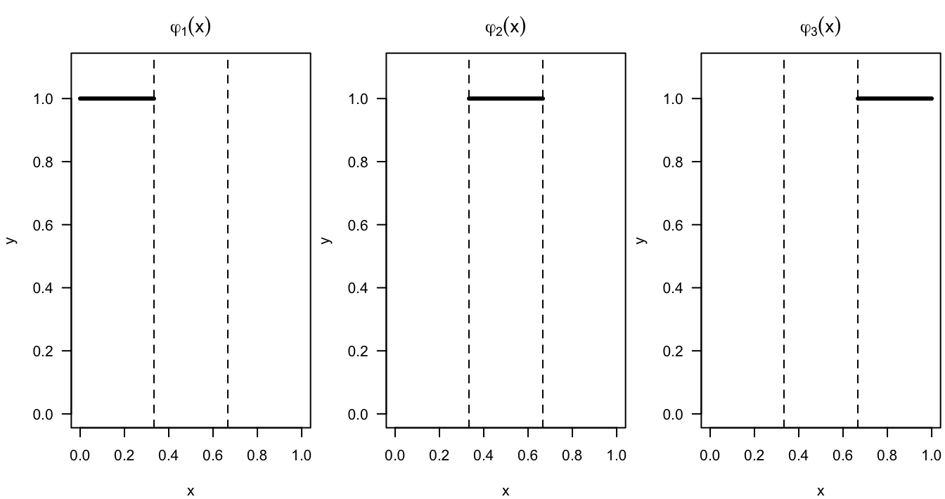
Figure 9.1: Basis functions for a regressogram with the following 3 bins: [0,1/3), [1/3, 2/3), [2/3, 1)
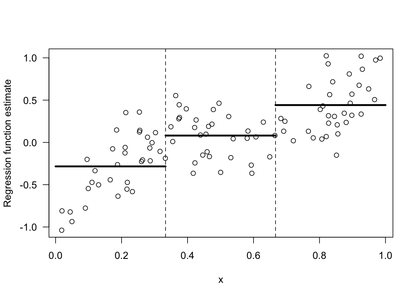
Figure 8.1: Regressogram estimate of a regression function with 3 bins.
13.1.2 Piecewise Linear Estimates
Instead of a piecewise constant estimate of \(m(x)\), we could use an estimate which is piecewise linear by using the following \(2p\) basis functions \[\begin{eqnarray} \varphi_{1}(x) &=& I(x \in B_{1}) \nonumber \\ &\vdots& \nonumber \\ \varphi_{p}(x) &=& I(x \in B_{p}) \nonumber \\ \varphi_{p+1}(x) &=& x I(x \in B_{1}) \nonumber \\ &\vdots& \nonumber \\ \varphi_{2p}(x) &=& x I(x \in B_{p}) \nonumber \end{eqnarray}\] if we now let \(p = D_{n}\) denote the number of “bins”.
The figure below shows an example of a regression function that is piecewise linear with 3 different bins.
While a piecewise linear model is perhaps a more flexible method than the regressogram, the piecwise linear model will still have big jumps at the bin boundaries and have an overall unpleasant appearance.

Figure 13.1: Example of a regression function estimate that is piecewise linear within 3 bins.
13.1.3 Piecewise Cubic Estimates
If we wanted to allow for more flexible forms of the regression function estimate within each bin we could fit a higher order polynomial model within each bin.
That is, the regression function estimate within the \(k^{th}\) bin will have the form \[\begin{equation} \hat{m}(x)I(x \in B_{k}) = \hat{\beta}_{0k} + \hat{\beta}_{1k}x + \hat{\beta}_{2k}x^{2} + \hat{\beta}_{3k}x^{3} \nonumber \end{equation}\]
To fit a piecewise cubic model with \(p\) bins, we would need the following \(4p\) basis functions \[\begin{eqnarray} \varphi_{1}(x) &=& I(x \in B_{1}), \ldots, \varphi_{p}(x) = I(x \in B_{p}) \nonumber \\ \varphi_{p+1}(x) &=& xI(x \in B_{1}), \ldots, \varphi_{2p}(x) = xI(x \in B_{p}) \nonumber \\ \varphi_{2p+1}(x) &=& x^{2}I(x \in B_{1}), \ldots, \varphi_{3p}(x) = x^{2}I(x \in B_{p}) \nonumber \\ \varphi_{3p+1}(x) &=& x^{3}I(x \in B_{1}), \ldots, \varphi_{4p}(x) = x^{3}I(x \in B_{p}) \nonumber \\ \end{eqnarray}\]
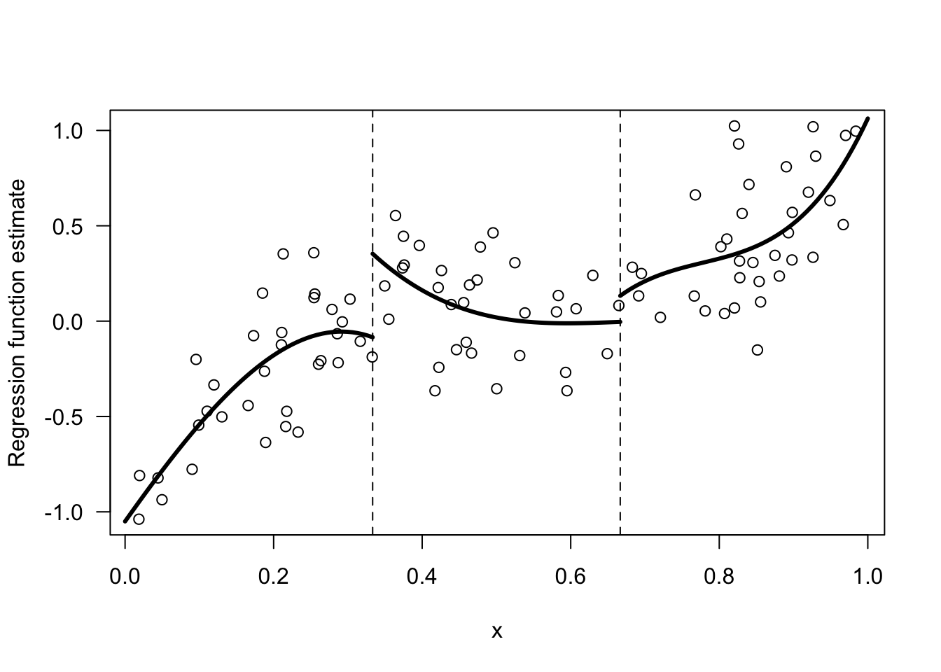
Figure 13.2: Example of a regression function estimate that is piecewise cubic within 3 bins.
13.2 Piecewise Linear Estimates with Continuity (Linear Splines)
In the spline world, one typically talks about “knots” rather than “bins”.
You can think of knots as the dividing points between the bins.
We will let \(u_{1} < u_{2} < \ldots < u_{q}\) denote the choice of knots.
The bins corresponding to this set of knots would then be \(B_{1} = (-\infty, u_{1}), B_{2} = [u_{1}, u_{2}), B_{3} = [u_{2}, u_{3}), \ldots, B_{q+1} = [u_{q}, \infty)\).
In other words, \(q\) knots defines \(B_{q+1}\) “bins” of the form \(B_{k} = [u_{k-1}, u_{k+1})\), for \(k = 2, \ldots, q\).
Let’s return to the piecewise linear estimate shown in Figure 13.1. This has two knots \(u_{1} = 1/3\) and \(u_{2} = 2/3\) and hence \(3\) bins.
Also, this piecewise linear model has \(6\) parameters. If we let \((\beta_{0k}, \beta_{1k})\) denote the intercept and slope parameters for the \(k^{th}\) bin, there are \(6\) parameters in total because we have \(3\) bins, and we could write a piecewise linear model as \[\begin{equation} m(x) = \begin{cases} \beta_{01} + \beta_{11}x & \text{ if } x < u_{1} \nonumber \\ \beta_{02} + \beta_{12}x & \text{ if } u_{1} \leq x < u_{2} \nonumber \\ \beta_{03} + \beta_{13}x & \text{if } x \geq u_{2} \end{cases} \end{equation}\]
We can make the estimated regression function look better by ensuring that it is continuous and does not have discontinuities at the knots.
To make the estimated regression curve continuous, we just need to make sure it is continuous at the knots.
That is, the regression coefficients need to satisfy the following two constraints: \[\begin{equation} \beta_{01} + \beta_{11}u_{1} = \beta_{02} + \beta_{12}u_{1} \qquad \textrm{and} \qquad \beta_{02} + \beta_{12}u_{2} = \beta_{03} + \beta_{03}u_{2} \nonumber \end{equation}\]
Because we have two linear constraints, we should expect that the number of “free parameters” in a piecewise linear model with continuity constraints should equal \(6 - 2 = 4\).
Indeed, if we use the fact that under the continuity constraints: \(\beta_{02} = \beta_{01} + \beta_{11}u_{1} - \beta_{12}u_{1}\) and \(\beta_{03} = \beta_{02} + \beta_{12}u_{2} - \beta_{13}u_{2}\), then we can rewrite the piecewise linear model as \[\begin{equation} m(x) = \begin{cases} \beta_{01} + \beta_{11}x & \text{ if } x < u_{1} \nonumber \\ \beta_{01} + \beta_{11}x + (\beta_{12} - \beta_{11})(x - u_{1}) & \text{ if } u_{1} \leq x < u_{2} \nonumber \\ \beta_{01} + \beta_{11}x + (\beta_{12} - \beta_{11})(x - u_{1}) + (\beta_{13} - \beta_{12})(x - u_{2}) & \text{ if } x \geq u_{2} \end{cases} \end{equation}\]
We can rewrite the above more compactly as: \[\begin{equation} m(x) = \beta_{01} + \beta_{11}x + (\beta_{12} - \beta_{11})(x - u_{1})_{+} + (\beta_{13} - \beta_{12})(x - u_{2})_{+} \nonumber \end{equation}\] where \((x - u_{1})_{+} = \max\{ x - u_{1}, 0\}\).
So, the functions \(\varphi_{0}(x) = 1\), \(\varphi_{1}(x) = x\), \(\varphi_{2}(x) = (x - u_{1})_{+}\), \(\varphi_{3}(x) = (x - u_{2})_{+}\) form a basis for the set of piecewise linear function with continuity constraints and knots \(u_{1}\) and \(u_{2}\).
In general, a linear spline with \(q\) knots \(u_{1} < u_{2} < \ldots < u_{q}\) is a funcion \(m(x)\) that can be expressed as \[\begin{equation} m(x) = \beta_{0} + \beta_{1}x + \sum_{k=1}^{q} \beta_{k+1} (x - u_{k})_{+} \nonumber \end{equation}\]
So, the following \(q + 2\) functions form a basis for the set of linear splines with knots \(u_{1} < u_{2} < \ldots < u_{q}\) \[\begin{eqnarray} \varphi_{0}(x) &=& 1 \nonumber \\ \varphi_{1}(x) &=& x \nonumber \\ \varphi_{2}(x) &=& (x - u_{1})_{+} \nonumber \\ \varphi_{3}(x) &=& (x - u_{2})_{+} \nonumber \\ &\vdots& \nonumber \\ \varphi_{q + 1}(x) &=& (x - u_{q})_{+} \nonumber \end{eqnarray}\]
Hence, if we want to fit a linear spline with \(q\) knots, we will need to estimate \(q + 2\) parameters.
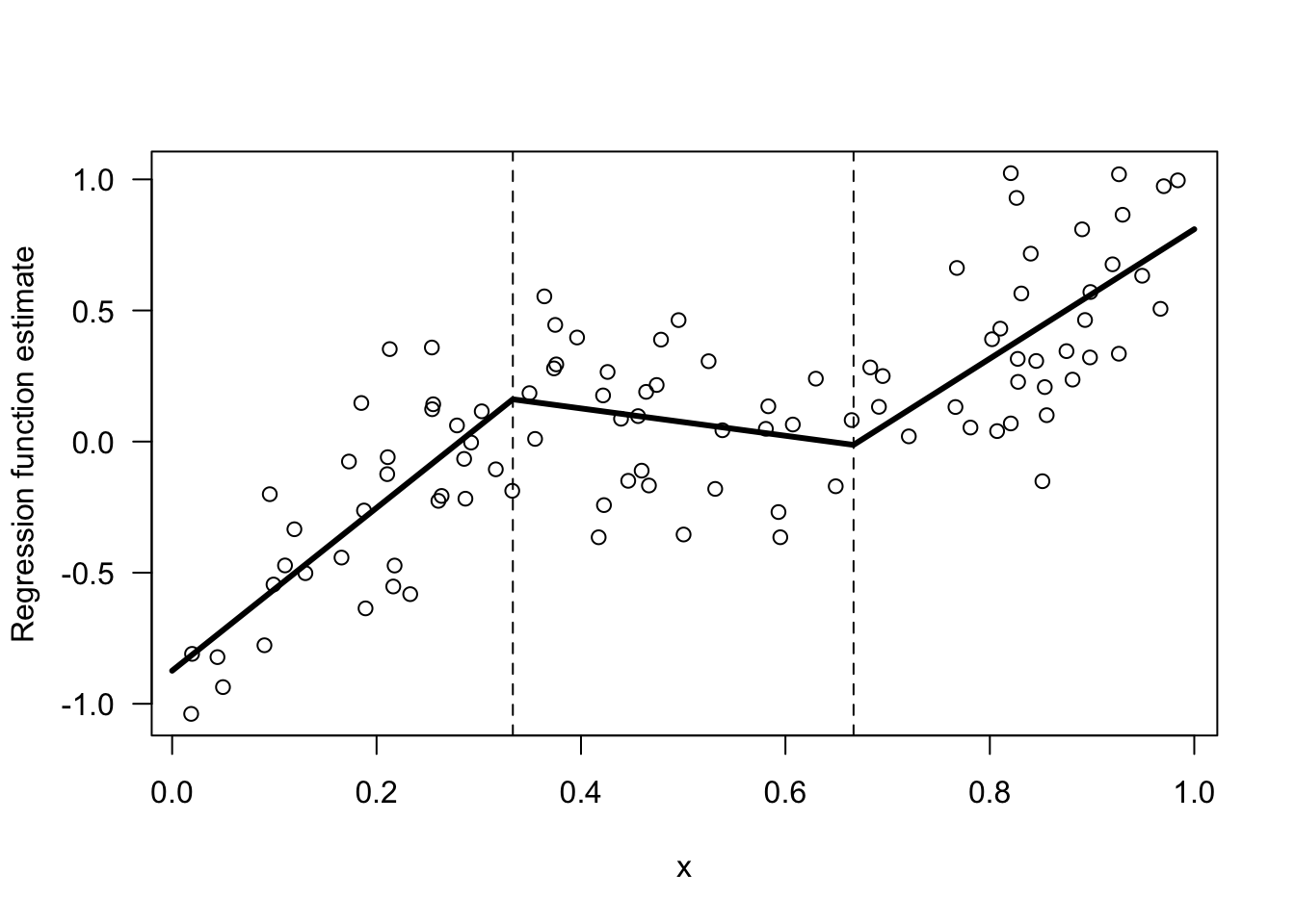
Figure 12.1: A linear spline with knots at 1/3 and 2/3. A linear spline is a piecewise linear function that is constrained to be continuous.
13.3 Cubic Splines and Regression with Splines
13.3.1 Example: Smooth Piecewise Cubic Model with 2 Knots
Let us go back to the piecewise cubic model shown in Figure 13.2.
This model assumes that the regression function is of the form: \[\begin{equation} m(x) = \begin{cases} \beta_{01} + \beta_{11}x + \beta_{21}x^{2} + \beta_{31}x^{3} & \text{ if } 0 < x < u_{1} \nonumber \\ \beta_{02} + \beta_{12}x + \beta_{22}x^{2} + \beta_{32}x^{3} & \text{ if } u_{1} \leq x < u_{2} \nonumber \\ \beta_{03} + \beta_{13}x + \beta_{23}x^{2} + \beta_{33}x^{3} & \text{ if } 1 > x \geq u_{2} \end{cases} \end{equation}\] Notice that this model has 12 parameters.
Like in the linear spline example, if we wanted to make this piecewise cubic model continuous at the knots \(u_{1}\) and \(u_{2}\) we would need to impose the following constraints on the coefficients \(\beta_{jk}\): \[\begin{eqnarray} \beta_{01} + \beta_{11}u_{1} + \beta_{21}u_{1}^{2} + \beta_{31}u_{1}^{3} &=& \beta_{02} + \beta_{12}u_{1} + \beta_{22}u_{1}^{2} + \beta_{32}u_{1}^{3} \nonumber \\ \beta_{02} + \beta_{12}u_{2} + \beta_{22}u_{2}^{2} + \beta_{21}u_{2}^{3} &=& \beta_{03} + \beta_{13}u_{2} + \beta_{23}u_{2}^{2} + \beta_{33}u_{2}^{3} \tag{13.1} \end{eqnarray}\]
However, only forcing the piecewise cubic model to be continuous is not enough if we want a smooth estimate for the regression function that will not have obvious changes at the knots.
We actually need the first and the second derivatives of the function to be continuous if we want a function that is smooth and does not have changes at the knots that we can detect visually.
So, for the example that we have in Figure 13.2 with the knots \(u_{1}\) and \(u_{2}\), we need to enforce the additional four constraints: \[\begin{eqnarray} \beta_{11} + 2\beta_{21}u_{1} + 3\beta_{31}u_{1}^{2} &=& \beta_{12} + 2\beta_{22}u_{1} + 3\beta_{32}u_{1}^{2} \nonumber \\ \beta_{12} + 2\beta_{22}u_{2} + 3\beta_{21}u_{2}^{2} &=& \beta_{13} + 2\beta_{23}u_{2} + 3\beta_{33}u_{2}^{2} \nonumber \\ 2\beta_{21} + 6\beta_{31}u_{1} &=& 2\beta_{22} + 6\beta_{32}u_{1} \nonumber \\ 2\beta_{22} + 6\beta_{21}u_{2} &=& 2\beta_{23} + 6\beta_{33}u_{2} \nonumber \end{eqnarray}\]
Hence, the piecewise cubic model that has the two continuity constraints (13.1) and the four first and second derivative constraints will have \(12 - 2 - 4 = 6\) parameters in total.
In a similar way to how we derived the basis for the linear spline with knots \(u_{1}\) and \(u_{2}\), you can show that the following \(6\) functions form a basis for the set of piecewise cubic functions with knots \(u_{1}\) and \(u_{2}\) that are continuous and have continuous first and second derivatives: \[\begin{eqnarray} \varphi_{0}(x) &=& 1 \qquad \varphi_{1}(x) = x \qquad \varphi_{2}(x) = x^{2} \qquad \varphi_{3}(x) = x^{3} \nonumber \\ \varphi_{4}(x) &=& (x - u_{1})_{+}^{3} \qquad \varphi_{5}(x) = (x - u_{2})_{+}^{3} \nonumber \end{eqnarray}\]
13.3.2 Cubic Splines
The above example with knots \(u_{1}\) and \(u_{2}\) is an example of a cubic spline.
Definition: A cubic spline with knots \(u_{1} < u_{2} < \ldots < u_{q}\) is a function \(f(x)\) such that
- \(f(x)\) is a cubic function over each of the intervals \((-\infty, u_{1}], [u_{1}, u_{2}], \ldots, [u_{q-1}, u_{q}], [u_{q}, \infty)\).
- \(f(x)\), \(f'(x)\), and \(f''(x)\) are all continuous functions.
One basis for the set of cubic splines with knots \(u_{1} < u_{2} < \ldots < u_{q}\) is the following truncated power basis which consists of \(q + 4\) basis functions: \[\begin{eqnarray} \varphi_{0}(x) &=& 1 \quad \varphi_{1}(x) = x \quad \varphi_{2}(x) = x^{2} \quad \varphi_{3}(x) = x^{3} \nonumber \\ \varphi_{k+3}(x) &=& (x - u_{k})_{+}^{3}, \quad k=1,\ldots, q \end{eqnarray}\]
A common basis for the set of cubic splines with knots \(u_{1} < u_{2} < \ldots < u_{q}\) is the B-spline basis.
Using the B-spline basis functions is mathematically equivalent to using the truncated power basis functions. Mathematically, using either basis would give you the same fitted curve.
However, there are computational advantages to using the B-spline basis functions, and using the B-spline seems to be much more common in software implementations of spline fitting procedures.
For a cubic spline with knots \(u_{1}, \ldots, u_{q}\), we will let the following \(q + 4\) denote the corresponding set of B-spline basis functions \[\begin{equation} \varphi_{1, B}(x), \ldots, \varphi_{q+4, B}(x) \nonumber \end{equation}\]
13.3.3 Estimating the Coefficients of a Cubic Spline
When fitting a cubic spline, we assume that the knots \(\mathbf{u} = (u_{1}, u_{2}, \ldots, u_{q})\) are fixed first.
Because the B-spline functions form a basis for the set of cubic splines with these knots, we can assume that our estimated regression function will have the form \[\begin{equation} m(x) = \sum_{k=1}^{q + 4} \beta_{k}\varphi_{k,B}(x) \nonumber \end{equation}\]
To find the best coeffients \(\beta_{k}\) in this cubic spline model, we will minimize the residual sum-of-residuals-squared criterion \[\begin{equation} \sum_{i=1}^{n} \Big( Y_{i} - \hat{m}(x_{i}) \Big)^{2} = \sum_{i=1}^{n} \Big( Y_{i} - \sum_{k=1}^{q + 4} \beta_{k}\varphi_{k,B}(x_{i}) \Big)^{2} \end{equation}\]
Finding the coefficients \(\hat{\beta}_{1}, \ldots, \hat{\beta}_{q+4}\) that minimize this sum-of-residuals-squared criterion can be viewed as solving a regression problem with response vector \(\mathbf{Y} = (Y_{1}, \ldots, Y_{n})\) and “design matrix” \(\mathbf{X}_{\mathbf{u}}\) \[\begin{equation} \mathbf{X}_{\mathbf{u}} = \begin{bmatrix} \varphi_{1, B}(x_{1}) & \varphi_{2, B}(x_{1}) & \ldots & \varphi_{q+4, B}(x_{1}) \\ \varphi_{1, B}(x_{2}) & \varphi_{2, B}(x_{2}) & \ldots & \varphi_{q+4,B}(x_{2}) \\ \vdots & \vdots & \ddots & \vdots \\ \varphi_{1,B}(x_{n}) & \varphi_{2,B}(x_{n}) & \ldots & \varphi_{q+4,B}(x_{n}) \end{bmatrix} \nonumber \end{equation}\]
When written in this form, the vector of estimated regression coeffients can be expressed as \[\begin{equation} \begin{bmatrix} \hat{\beta}_{1} \\ \hat{\beta}_{2} \\ \vdots \\ \hat{\beta}_{q + 4} \end{bmatrix} = (\mathbf{X}_{\mathbf{u}}^{T}\mathbf{X}_{\mathbf{u}})^{-1}\mathbf{X}_{\mathbf{u}}^{T}\mathbf{Y} \nonumber \end{equation}\] and hence the vector of fitted values \(\hat{\mathbf{m}} = \big( \hat{m}(x_{1}), \ldots, \hat{m}(x_{n}) \big)\) can be written as \[\begin{equation} \hat{\mathbf{m}} = \mathbf{X}_{\mathbf{u}}(\mathbf{X}_{\mathbf{u}}^{T}\mathbf{X}_{\mathbf{u}})^{-1}\mathbf{X}_{\mathbf{u}}^{T}\mathbf{Y} \nonumber \end{equation}\]
13.3.4 An example in R
- Regression splines can be fitted in R by using the
splinespackage
- The
bsfunction from thesplinespackage is useful for fitting a linear or cubic spline. This function generates the B-spline “design” matrix \(\mathbf{X}_{\mathbf{u}}\) described above.
x- vector of covariates values. This can also just be the name of a variable whenbsis used inside thelmfunction.df- the “degrees of freedom”. For a cubic spline this is actually \(q + 3\) rather than \(q + 4\). If you just enterdf, thebsfunction will pick the knots for you.knots- the vector of knots. If you don’t want to pick the knots, you can just enter a number for thedf.degree- the degree of the piecewise polynomial. degree=1 for a linear spline and degree=3 for a cubic spline.
As an example of what the
bsfunction returns, suppose we input the vector of covariates \((x_{1}, \ldots, x_{10}) = (1, 2, \ldots, 10)\) with knots \(u_{1} = 3.5\) and \(u_{2} = 6.5\).The
bsfunction will return the “design matrix” \(\mathbf{X}_{\mathbf{u}}\) for this setup without the intercept column. When degree is 3, the dimensions of \(\mathbf{X}_{\mathbf{u}}\) should be \(10 \times 6\) (because in this case \(q = 2\)). So, thebsfunction will return a \(10 \times 5\) matrix (because the first column of \(\mathbf{X}_{u}\) is dropped bybs):
## [1] 10 5## 1 2 3 4 5
## [1,] 0.00000 0.000 0.00000 0.000000 0
## [2,] 0.60813 0.168 0.00808 0.000000 0
## [3,] 0.45779 0.470 0.06465 0.000000 0
## [4,] 0.17218 0.612 0.21463 0.000986 0
## [5,] 0.03719 0.515 0.42131 0.026627 0
## [6,] 0.00138 0.309 0.56631 0.123274 0Let’s try an example with a linear spline to see how to use the
bsfunction to fit a spline within thelmfunction.We will use the
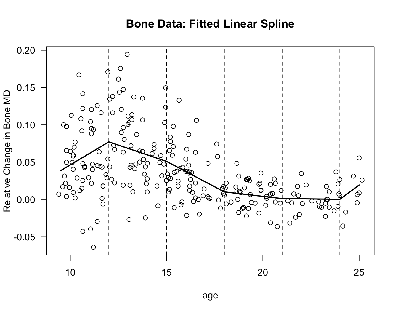
bonedata again with age as the covariate. We will use the knots \(\mathbf{u} = (12, 15, 18, 21, 24)\).
knot.seq <- c(12, 15, 18, 21, 24)
linspline.bone <- lm(spnbmd ~ bs(age, knots=knot.seq, degree=1), data=bonedat)
Because we are using \(5\) knots, based on our discussion in Section 12.2 we should expect that there should be \(7\) columns in the design matrix \(\mathbf{X}_{u}\) for this linear spline model.
You can check this by using the following
Rcode:
## [1] 261 7- If you want to compute the estimated spline function \(\hat{m}(t_{j})\) at a sequence of points \(t_{1}, \ldots, t_{l}\),
you can use the
predictfunction on the fittedlmobject. This is done with the following code for the points \(9.5, 10, 10.5, 11, \ldots, 24.5, 25\).
tt <- seq(9.5, 25, by=0.5)
plot(bonedat$age, bonedat$spnbmd, xlab="age", ylab="Relative Change in Bone MD",
     main="Bone Data: Fitted Linear Spline", las=1)
lines(tt, predict(linspline.bone, data.frame(age=tt)), lwd=2)
for(k in 1:5) {
    ## Plot vertical lines at the knots
    abline(v=knot.seq[k], lty=2)
}
Now let’s try fitting a cubic spline model to the bone data.
The procedure is almost exactly the same as fitting the linear spline model. We only need to change
degree=1todegree=3in thebsfunction.We will use the same knots as we did for the linear spline.
knot.seq <- c(12, 15, 18, 21, 24)
cubspline.bone <- lm(spnbmd ~ bs(age, knots=knot.seq, degree=3), data=bonedat)
Because we are using \(5\) knots, we should expect that there will be \(5 + 4 = 9\) columns in the design matrix \(\mathbf{X}_{u}\) for this cubic spline model.
You can check this by using the following
Rcode:
## [1] 261 9- Using
predictagain, we will compute the estimated regression function \(\hat{m}(x)\) at the points: \(9.5, 9.6, \ldots, 24.9, 25\) and plot the result.
tt <- seq(9.5, 25, by=0.1)
plot(bonedat$age, bonedat$spnbmd, xlab="age", ylab="Relative Change in Bone MD",
     main="Bone Data: Fitted Cubic Spline", las=1)
lines(tt, predict(cubspline.bone, data.frame(age=tt)), lwd=2)
for(k in 1:5) {
    ## Plot vertical lines at the knots
    abline(v=knot.seq[k], lty=2)
}
13.3.5 Natural Cubic Splines
Cubic splines can often have highly variable behavior near the edges of the data (i.e., for points near the smallest and largest \(x_{i}\)).
One approach for addressing this problem is to use a spline which is linear for both \(x < u_{1}\) and \(x > u_{q}\).
A natural cubic spline is a function that is still a piecewise cubic function over each of the intervals \([u_{j}, u_{j+1}]\) for \(j=1, \ldots, q-1\), but is linear for \(x < u_{1}\) and \(x > u_{q}\). A natural cubic spline is still assumed to satisfy all of the continuity and derivative continuity conditions of the usual cubic spline.
Natural cubic splines are also useful for fitting smoothing splines.
Because we are using linear rather than cubic functions in the regions \((-\infty, u_{1})\) and \((u_{q}, \infty)\) this should reduce the number of necessary basis functions by \(4\) (so we would only need \(q\) rather \(q + 4\) basis functions).
Indeed, one basis for the set of natural cubic splines with knots \(u_{1}, \ldots, u_{q}\) is the following collection of \(q\) basis functions: \[\begin{equation} N_{1}(x) = 1 \qquad N_{2}(x) = x \qquad N_{k+2} = d_{k}(x) - d_{q-1}(x), k = 1, \ldots, q-2, \nonumber \end{equation}\] where the functions \(d_{k}(x)\) are defined as \[\begin{equation} d_{k}(x) = \frac{ (x - u_{k})_{+}^{3} - (x - u_{q})_{+}^{3} }{ u_{q} - u_{k}} \nonumber \end{equation}\]
natural.cubspline.bone <- lm(spnbmd ~ ns(age, df=8), data=bonedat)
tt <- seq(9.5, 25, by=0.1)
plot(bonedat$age, bonedat$spnbmd, xlab="age", ylab="Relative Change in Bone MD",
     main="Bone Data: Fitted Natural Cubic Spline", las=1)
lines(tt, predict(natural.cubspline.bone, data.frame(age=tt)), lwd=2)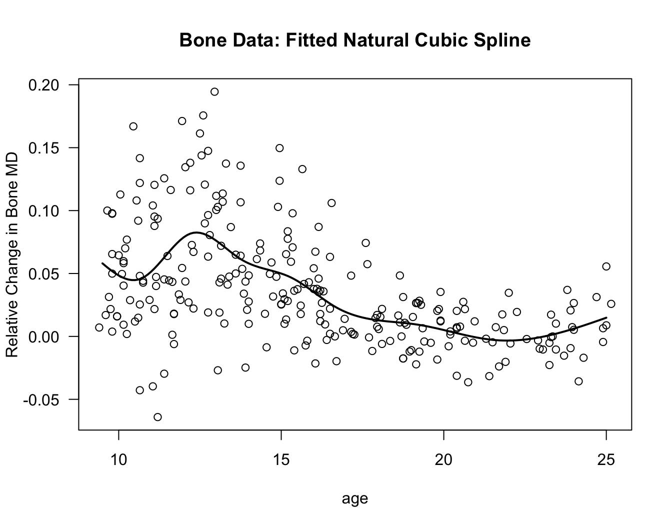
13.4 Smoothing Splines
When we used cubic splines for regression, we placed knots at a number of fixed points in between the smallest and largest \(x_{i}\) values.
With what are referred to as “smoothing splines” every point \(x_{i}\) is treated as a potential knot, and the overall smoothness of the regression function estimate is determined through penalizing the roughness of the function.
Motivation for smoothing splines can come from considering the following minimization problem:
- For \(\lambda \geq 0\), suppose we want to find the function \(m(x)\) which solves the optimization problem: \[\begin{equation} \textrm{minimize:} \quad \sum_{i=1}^{n} \{ Y_{i} - m( x_{i} ) \}^{2} + \lambda \int \{ m''(x) \}^{2} dx \tag{13.2} \end{equation}\] subject to the constraint that \(m'(x)\) and \(m''(x)\) are both continuous.
The second derivative \(m''(x)\) represents the curvature of \(m\) at \(x\). So, the penalty \(\int \{ m''(x) \}^{2} dx\) is like an average squared curvature of the function \(m(x)\).
If \(\lambda = 0\), then the function \(m(x)\) which minimizes (13.2) is any function such that \(m(x_{i}) = Y_{i}\) for each \(i\). This will usually be an extremely “wiggly” function.
If \(\lambda = \infty\), then we want a function \(m(x)\) such that \(m''(x) = 0\) for all \(x\). The best function in this case would be a linear function \(m(x) = \beta_{0} + \beta_{1}x\).
By choosing \(0 < \lambda < \infty\), we will get a function that can be nonlinear and capture some curvature but cannot be extremely “wiggly”.
It is possible to show that the function \(\hat{m}_{\lambda}(x)\) which minimizes (13.2) is a natural cubic spline with \(n\) knots at the covariate values \((x_{1}, \ldots, x_{n})\).
So, we can restrict our search to functions which can be written as \[\begin{equation} m(x) = \sum_{j=1}^{n} \beta_{j}N_{j}(x), \nonumber \end{equation}\] where \(N_{1}(x), \ldots, N_{n}(x)\) is the set of basis functions for the set of natural cubic splines with these knots.
So, assuming that \(m(x) = \sum_{j=1}^{n} \beta_{j}N_{j}(x)\), we can re-write the minimization problem as \[\begin{equation} \textrm{minimize:}_{\beta_{1}, \ldots, \beta_{n}} \sum_{i = 1}^{n} \{ Y_{i} - \sum_{j=1}^{n} \beta_{j}N_{j}(x_{i}) \}^{2} + \lambda \sum_{j=1}^{n} \sum_{k=1}^{n} \beta_{j}\beta_{k} \int N_{j}''(x) N_{k}''(x) dx \nonumber \end{equation}\]
In matrix-vector notation, this minimization problem can be written as \[\begin{equation} \textrm{minimize:}_{\boldsymbol\beta} \quad (\mathbf{Y} - \mathbf{N}\boldsymbol\beta)^{T}(\mathbf{Y} - \mathbf{N}\boldsymbol\beta) + \lambda \boldsymbol\beta^{T}\boldsymbol\Omega\boldsymbol\beta, \tag{13.3} \end{equation}\] where \(\mathbf{N}\) is the \(n \times n\) matrix whose \((j,k)\) element is \(N_{k}(x_{j})\) and \(\boldsymbol\Omega\) is the \(n \times n\) matrix whose \((j,k)\) element is \(\Omega_{jk} = \int N_{j}''(x)N_{k}''(x) dx\).
The vector of coefficients which solves the minimization problem (13.3) is given by \[\begin{equation} \hat{\boldsymbol\beta} = \begin{bmatrix} \hat{\beta}_{1} \\ \vdots \\ \hat{\beta}_{n} \end{bmatrix} = (\mathbf{N}^{T}\mathbf{N} + \lambda \boldsymbol\Omega)^{-1}\mathbf{N}^{T}\mathbf{Y} \nonumber \end{equation}\]
13.5 Knot/Penalty Term Selection for Splines
For both regression splines and smoothing splines, we can write the vector of fitted values \(\hat{\mathbf{m}} = \big( \hat{m}(x_{1}), \ldots, \hat{m}(x_{n}) \big)\) as \[\begin{equation} \hat{\mathbf{m}} = \mathbf{A}\mathbf{Y}, \nonumber \end{equation}\] for an appropriately chosen \(n \times n\) matrix \(\mathbf{A}\).
For the case of a cubic regression spline with fixed knot sequence \(\mathbf{u} = (u_{1}, \ldots, u_{q})\), we have that \(\hat{\mathbf{m}} = \mathbf{A}_{\mathbf{u}}\mathbf{Y}\) where \[\begin{equation} \mathbf{A}_{\mathbf{u}} = \mathbf{X}_{\mathbf{u}}(\mathbf{X}_{\mathbf{u}}^{T}\mathbf{X}_{\mathbf{u}})^{-1}\mathbf{X}_{\mathbf{u}}^{T} \end{equation}\] Note that, in this case, \[\begin{equation} \textrm{tr}( \mathbf{A}_{\mathbf{u}} ) = \textrm{tr}( \mathbf{X}_{\mathbf{u}}(\mathbf{X}_{\mathbf{u}}^{T}\mathbf{X}_{\mathbf{u}})^{-1}\mathbf{X}_{\mathbf{u}}^{T} ) = \textrm{tr}( (\mathbf{X}_{\mathbf{u}}^{T}\mathbf{X}_{\mathbf{u}})^{-1}\mathbf{X}_{\mathbf{u}}^{T}\mathbf{X}_{u} ) = q + 4 \end{equation}\]
For the case of a smoothing spline with penalty term \(\lambda > 0\), we have that \(\hat{\mathbf{m}} = \mathbf{A}_{\lambda}\mathbf{Y}\) where \[\begin{equation} \mathbf{A}_{\lambda} = \mathbf{N}(\mathbf{N}^{T}\mathbf{N} + \lambda\boldsymbol\Omega)^{-1}\mathbf{N}^{T} \nonumber \end{equation}\]
13.5.1 The Cp Statistic
As with kernel and local regression method described in Chapter 12, the \(C_{p}\) statistic is defined as the mean residual sum of squares plus a penalty which depends on the matrix \(\mathbf{A}\).
In the context of regression splines where \(\hat{\mathbf{m}} = \mathbf{A}_{\mathbf{u}}\mathbf{Y}\), the \(C_{p}\) statistic can be written as: \[\begin{eqnarray} C_{p}(q) &=& \frac{1}{n}\sum_{i=1}^{n}\{ Y_{i} - \hat{m}(x_{i}) \}^{2} + \frac{2\hat{\sigma}^{2}}{n}\textrm{tr}(\mathbf{A}_{u}) \nonumber \\ &=& \frac{1}{n}\sum_{i=1}^{n}\{ Y_{i} - \hat{m}(x_{i}) \}^{2} + \frac{2\hat{\sigma}^{2}(q + 4)}{n} \nonumber \end{eqnarray}\]
In the context of smoothing splines where \(\hat{\mathbf{m}} = \mathbf{A}_{\lambda}\mathbf{Y}\), the \(C_{p}\) statistic can be written as \[\begin{eqnarray} C_{p}(\lambda) &=& \frac{1}{n}\sum_{i=1}^{n}\{ Y_{i} - \hat{m}(x_{i}) \}^{2} + \frac{2\hat{\sigma}^{2}}{n}\textrm{tr}(\mathbf{A}_{\lambda}) \nonumber \\ &=& \frac{1}{n}\sum_{i=1}^{n}\{ Y_{i} - \hat{m}(x_{i}) \}^{2} + \frac{2\hat{\sigma}^{2}}{n}\textrm{tr}\Big( (\mathbf{N}^{T}\mathbf{N} + \lambda\boldsymbol\Omega)^{-1}\mathbf{N}^{T}\mathbf{N} \Big) \nonumber \end{eqnarray}\]
13.5.2 Leave-one-out Cross-Validation
As mentioned in Chapter 12, the leave-one-out cross-validation can be expressed as a weighted sum-of-squared residuals with the weights coming from the diagonals of the “smoothing” matrix \(\mathbf{A}\).
For the smoothing spline, the leave-one-out cross-validation criterion is \[\begin{equation} \textrm{LOOCV}(\lambda) = \frac{1}{n}\sum_{i=1}^{n} \Big( \frac{ Y_{i} - \hat{m}_{\lambda}(x_{i})}{ 1 - a_{i}^{\lambda}( x_{i} ) } \Big)^{2} \nonumber \end{equation}\] where \(a_{i}^{\lambda}(x_{i})\) denotes the \(i^{th}\) diagonal of the matrix \(\mathbf{A}_{\lambda}\).
13.5.3 Generalized Cross-Validation
A criterion which we did not mention in Chapter 12 is Generalized Cross-Validation (GCV).
For the smoothing parameter \(\lambda\), the GCV criterion is defined as \[\begin{equation} \textrm{GCV}(\lambda) = \frac{1}{n}\sum_{i=1}^{n} \Big( \frac{ Y_{i} - \hat{m}_{\lambda}(x_{i})}{ 1 - \textrm{tr}(\mathbf{A}_{\lambda})/n } \Big)^{2} = \Big(\frac{n}{n - \textrm{tr}(\mathbf{A}_{\lambda})} \Big)^{2} \frac{1}{n} \sum_{i=1}^{n} \{Y_{i} - \hat{m}_{\lambda}(x_{i}) \}^{2} \nonumber \end{equation}\]
The GCV criterion can be seen as replacing the individual diagonal elements in the \(\textrm{LOOCV}\) criterion with their average value \(\textrm{tr}(\mathbf{A}_{\lambda})/n\).
GCV can often perform better when some of the diagonal elements of \(\mathbf{A}_{\lambda}\) are close to \(1\).
13.6 Fitting Smoothing Splines in R
- The
Rfunctionsmooth.splinewill fit smoothing splines.
x - the vector of covariate values.
y - the vector of responses.
df - the trace of the “smoother” matrix. This is the trace of the matrix \(\mathbf{A}_{\lambda} = \mathbf{N}(\mathbf{N}^{T}\mathbf{N} + \lambda\boldsymbol\Omega)^{-1}\mathbf{N}^{T}\). This must be less than or equal to \(n\) (where \(n\) here is the number of unique values of the \(x_{i}\)).
lambda - the value of \(\lambda\) in the matrix \(\mathbf{A}_{\lambda} = \mathbf{N}(\mathbf{N}^{T}\mathbf{N} + \lambda\boldsymbol\Omega)^{-1}\mathbf{N}^{T}\). Note that you should only enter one of the df or lambda arguments.
cv - the smooth.spline function will perform cross-validation whenever both the df and lambda arguments are left empty. When both of these arguments are left empty and
cv=FALSE, the function will use GCV to select the smoothing parameter. When both df and lambda are left empty andcv = TRUE, the function will use LOOCV to select the smoothing parameter.Notice that when only input the
xandyvectors, thesmooth.splinewill automatically use generalized cross-validation to select the smoothing parameter.
To see how to use the
smooth.splinefunction and how to use the \(C_{p}\) statistic, LOOCV, or GCV for selecting the smoothing parameter in smoothing splines or the number of knots in regression splines, we will again consider thebonedata.To start, let’s use the
smooth.splinefunction on the bone data using GCV to find the smoothing parameter:
ss.bone <- smooth.spline(x=bonedat$age, y=bonedat$spnbmd)

plot(bonedat$age, bonedat$spnbmd, las=1, pch=16, xlab="age",
     ylab="Relative Change in Bone MD", main="Bone Data: Smoothing Spline using GCV")
lines(ss.bone$x, ss.bone$y, lwd=3, col="red")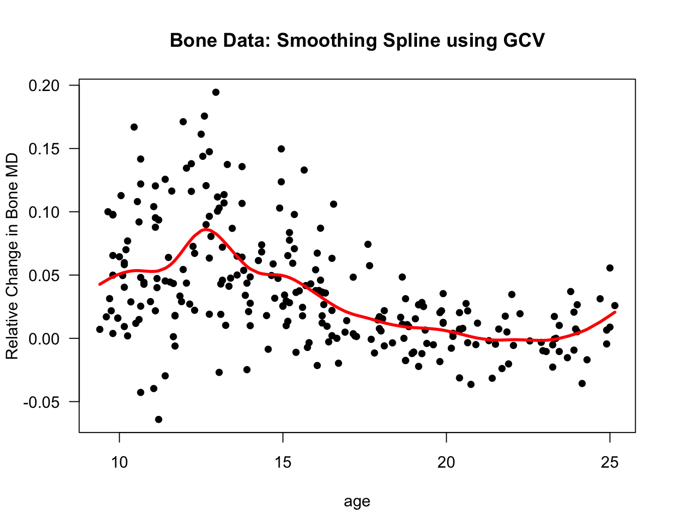
Figure 9.2: Smoothing spline fit for the bone data. This used the smooth.spline function with all the default settings.
- If you just type in
ss.bone, this will show the degrees of freedom used, the value of \(\lambda\) used, and the value of the GCV criterion for the chosen \(\lambda\)
## Call:
## smooth.spline(x = bonedat$age, y = bonedat$spnbmd)
##
## Smoothing Parameter  spar= 0.712  lambda= 0.000239 (15 iterations)
## Equivalent Degrees of Freedom (Df): 12.2
## Penalized Criterion (RSS): 0.222
## GCV: 0.00152
According to the GCV criterion, the best value for \(\lambda\) is about \(\lambda^{*} \approx 0.0002\) and the corresponding value for the degrees of freedom is \(df^{*} = \textrm{tr}(\mathbf{A}_{\lambda^{*}}) \approx 12.15\).
Using the LOOCV criterion, the best value for the degrees of freedom is \(13\).
## Warning in smooth.spline(x = bonedat$age, y = bonedat$spnbmd, cv = TRUE):
## cross-validation with non-unique 'x' values seems doubtful## Call:
## smooth.spline(x = bonedat$age, y = bonedat$spnbmd, cv = TRUE)
##
## Smoothing Parameter spar= 0.694 lambda= 0.000177 (13 iterations)
## Equivalent Degrees of Freedom (Df): 13
## Penalized Criterion (RSS): 0.219
## PRESS(l.o.o. CV): 0.0014913.6.1 Smoothing Parameter Selection for the Smoothing Spline with the Cp statistic
Suppose we wanted to find the best value of \(\textrm{tr}( \mathbf{A}_{\lambda})\) of the smoothing spline using the \(C_{p}\) statistic.
The first thing we want to find is an estimate of \(\sigma^{2}\) that we can keep fixed across different values of the smoothing parameter. Let’s use the same value of \(\hat{\sigma}^{2} = 0.0015\) that we used in Chapter 12:
- Now, let’s write a function that computes the \(C_{p}\) statistic for a smoothing spline model given that we input the data, the degrees of freedom \(\textrm{tr}(\mathbf{A}_{\lambda})\), and \(\hat{\sigma}^{2}\).
CpStatSmoothSpline <- function(x, y, df, sigsq.hat) {
  n <- length(x)
  ss.obj <- smooth.spline(x=x, y=y, df=df)
  ## Now, compute the vector of residuals from this fitted smoothing spline
  residu <- y - fitted(ss.obj)
  ans <- mean(residu^2) + (2*sigsq.hat/n)*df
  return(ans)
}- Now, compute the \(C_{p}\) statistic for values of the degrees of freedom between \(4\) and \(20\). From the plot of the \(C_{p}\) vs. the degrees of freedom it looks like the best value for the degrees of freedom is about \(12\)
df.seq <- seq(4, 20, by=.1)
nx <- length(df.seq)
Cp.seq <- numeric(nx)
for(k in 1:nx) {
    Cp.seq[k] <- CpStatSmoothSpline(x=bonedat$age, y=bonedat$spnbmd, df=df.seq[k],
                                    sigsq.hat=sigsq.est)
}

plot(df.seq, Cp.seq, ylab="CP Statistic", xlab="degrees of freedom",
    main="Bone Data: Cp(df) vs. df for the Smoothing Spline")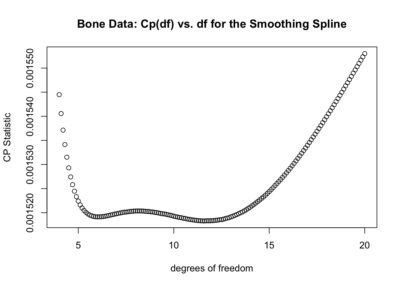
- More specifically, it’s about \(11.6\):
## [1] 11.613.6.2 Knot Selection for Regression Splines with the Cp statistic
Let’s go back to the regression spline methods we described in Section 12.3 also use the bone data to try to find the best number of knots for the case of regression splines.
We will consider knots \(u_{1}, \ldots, u_{q}\) that are computed automatically by the
bsfunction when we specify the degrees of freedom. These are based on the quantiles of the covariate \(x_{i}\). We will consider values of \(q\) between \(0\) and \(20\).
sigsq.hat <- .0015
n <- nrow(bonedat)

qqseq <- 0:20
Cp.seq <- rep(0, length(qqseq))
nq <- length(qqseq)
for(k in 1:nq) {
  q = qqseq[k]
  tt <- 1:q

  #uu <- 9.4 + (15.7/(q+1))*tt
  if(q == 0) {
    tmp <- lm(bonedat$spnbmd ~ bs(bonedat$age, df=q+3))
  } else {
    tmp <- lm(bonedat$spnbmd ~ bs(bonedat$age, df=q+3))
  }
  RSS <- mean((bonedat$spnbmd - tmp$fitted.values)^2)
  Cp.seq[k] <- RSS + (2*sigsq.hat*(q + 4))/n
}
plot(qqseq, Cp.seq, xlab="Number of Knots", ylab="Cp Statistic",
     main="Bone Data with Regression Splines: Cp Statistic for Different Number of Knots")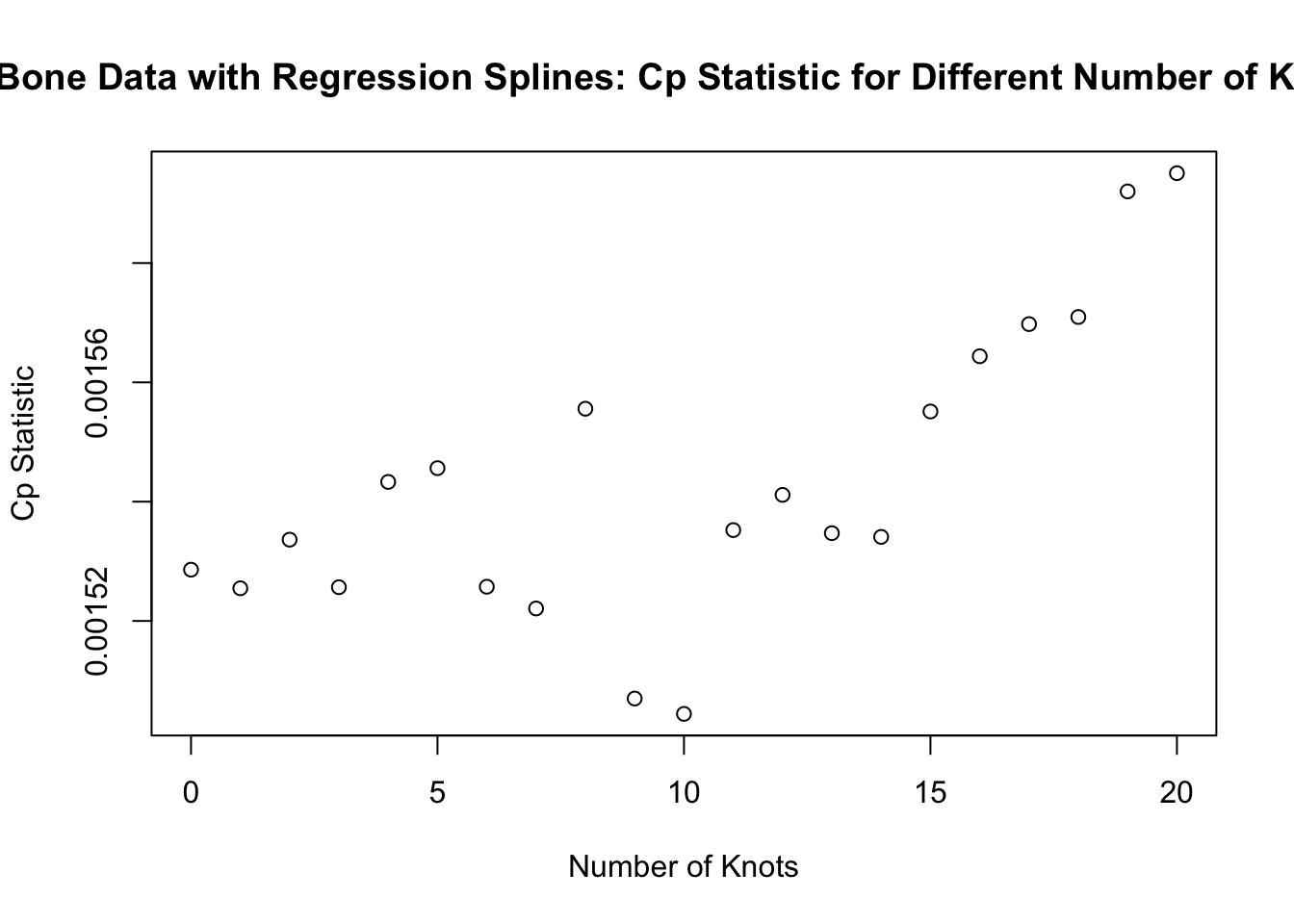
- From the plot, it looks like the best number of knots when using the \(C_{p}\) statistic is \(q = 10\).