Chapter 9 The Bootstrap

9.1 Introduction

• The jackknife and the bootstrap are nonparametric procedures that are mainly used for finding standard errors and constructing confidence intervals.

Why use the bootstrap?

1. To find better standard errors and/or confidence intervals when the standard approximations do not work very well.
2. To find standard errors and/or confidence intervals when you have no idea how to compute reasonable standard errors.

---

Example: Inference for \(e^{\mu}\)

• Suppose we have i.i.d. data \(X_{1}, \ldots, X_{n} \sim \textrm{Logistic}( \mu, s)\), meaning that \(E(X_{i}) = \mu\) and \(\textrm{Var}(X_{i}) = \sigma^{2} = s^{2}\pi^{2}/3\).

• Suppose our goal is to construct a confidence interval for the parameter \(\theta = e^{\mu}\).

• The traditional approach to constructing a confidence interval uses the fact that \[\begin{equation} \sqrt{n}\Big( e^{\bar{X}} - e^{\mu} \Big) \longrightarrow \textrm{Normal}(0, \sigma^{2}e^{2\mu}) \nonumber \end{equation}\] so that we can assume \(e^{\bar{X}}\) has a roughly Normal distribution with mean \(e^{\mu}\) and standard deviation \(\sigma e^{\mu}/\sqrt{n}\). This approximation is based on a Central Limit Theorem and “delta method” argument.

• The estimated standard error in this case is \[\begin{equation} \frac{\hat{\sigma}e^{\bar{X}}}{\sqrt{n}} \nonumber \end{equation}\]

• Using this Normal approximation for \(e^{\bar{X}}\), the \(95\%\) confidence interval for \(e^{\mu}\) is \[\begin{equation} \Big[ e^{\bar{X}} - 1.96 \times \frac{\hat{\sigma}e^{\bar{X}}}{\sqrt{n}}, e^{\bar{X}} + 1.96 \times \frac{\hat{\sigma}e^{\bar{X}}}{\sqrt{n}} \Big] \tag{9.1} \end{equation}\]

---

• For specific choices of \(n\), how good is the Normal approximation for the distribution of \(e^{\bar{X}}\)?

• The figure below shows a histogram for the simulated distribution of \(e^{\bar{X}}\) when \(n=50\). The density of the Normal approximation is also shown in this figure.

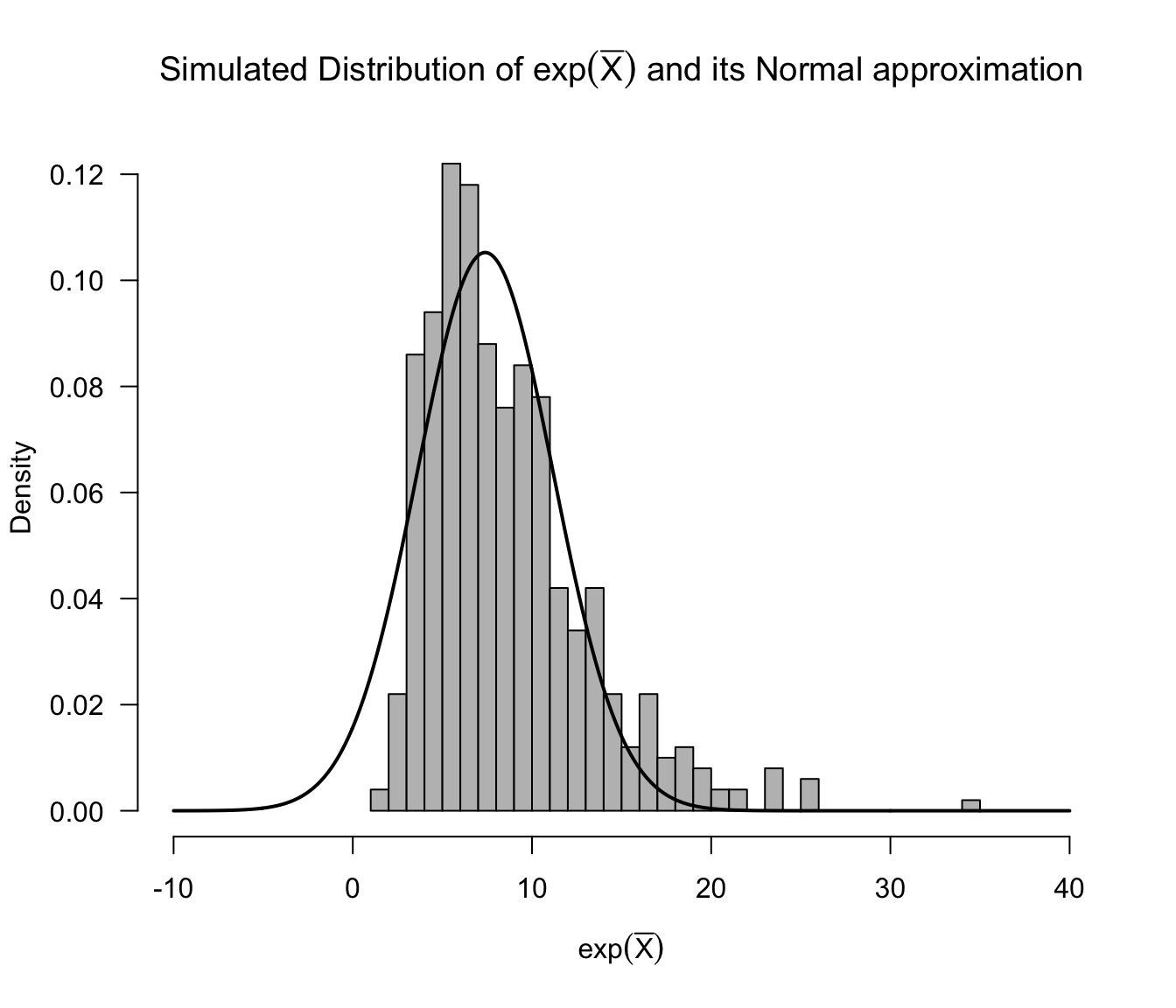
Figure 8.1: Histogram of simulated values of exp(sample mean) with density of the Normal approximation overlaid. This assumes n=50 and that the data are from a Logistic distribution with mu = 2 and s = 2.

• As we can see from the above histogram, the Normal approximation is not terrible. However, it really does not capture the skewness in the distribution of \(e^{\bar{X}}\) correctly.

• This could effect the coverage performance of confidence intervals which use Normal approximation (9.1).

• The bootstrap offers an alternative approach for constructing confidence intervals which does not depend on parametric approximations such as (9.1).

---

Example: Inference for the Correlation

• The sample correlation \(\hat{\rho}\) which estimates the correlation \(\rho = \textrm{Corr}(X_{i}, Y_{i})\) between \(X_{i}\) and \(Y_{i}\) is defined as \[\begin{equation} \hat{\rho} = \frac{\sum_{i=1}^{n}(X_{i} - \bar{X})(Y_{i} - \bar{Y})}{\sqrt{\sum_{i=1}^{n}(X_{i} - \bar{X})^{2}}\sqrt{\sum_{i=1}^{n}(Y_{i} - \bar{Y})}} \nonumber \end{equation}\]

• Even such a relatively straightforward estimate has a pretty complicated formula for the estimated standard error if you use a multivariate delta method argument: \[\begin{equation} \textrm{std.err}_{corr} = \Bigg\{ \frac{\hat{\rho}^{2}}{4n}\Bigg[ \frac{\hat{\mu}_{40}}{\hat{\mu}_{20}^{2}} + \frac{\hat{\mu}_{04}}{\hat{\mu}_{02}^{2}} + \frac{2\hat{\mu}_{22}}{\hat{\mu}_{20}\hat{\mu}_{02} } + \frac{4\hat{\mu}_{22}}{\hat{\mu}_{11}^{2}} - \frac{4\hat{\mu}_{31}}{\hat{\mu}_{11}\hat{\mu}_{20} } - \frac{4\hat{\mu}_{13}}{\hat{\mu}_{11}\hat{\mu}_{02} } \Bigg] \Bigg\}^{1/2} \tag{9.2} \end{equation}\] where \[\begin{equation} \hat{\mu}_{hk} = \sum_{i=1}^{n}(X_{i} - \bar{X})^{h}(Y_{i} - \bar{Y})^{k} \nonumber \end{equation}\]

• Another popular approach for constructing a confidence interval is to use Fisher’s “z-transformation” \[\begin{equation} z = \frac{1}{2} \ln\Big( \frac{1 + \hat{\rho}}{1 - \hat{\rho}} \Big) \tag{9.3} \end{equation}\] where it is argued that \(z\) has a roughly Normal distribution with mean \(\tfrac{1}{2}\ln\{ (1 + \rho)/(1 - \rho) \}\) and standard deviation \(1/\sqrt{n - 3}\).

---

• The bootstrap allows us to totally bypass the need to derive tedious formulas for the standard error such as (9.2) or bypass the need to use clever transformations such as (9.3).

• For many more complicated estimates deriving formulas such as (9.2) or transformations such as (9.3) may not even be feasible.

• The bootstrap provides an automatic way of constructing confidence intervals. You only need to be able to compute the estimate of interest.

9.2 Description of the Bootstrap

9.2.1 Description

• Suppose we have a statistic \(T_{n}\) that is an estimate of some quantity of interest \(\theta\).

• For example:
  • \(T_{n}\) - sample mean, \(\theta = E(X_{1})\).
  • \(T_{n}\) - sample correlation, \(\theta = \textrm{Corr}(X_{1}, Y_{1})\).
  • \(T_{n}\) - sample median, \(\theta = F^{-1}(1/2)\); that is, the true median.

• Typically, \(T_{n}\) can be represented as a function of our sample \(X_{1}, \ldots, X_{n}\) \[\begin{equation} T_{n} = h\Big( X_{1}, \ldots, X_{n} \Big) \nonumber \end{equation}\]

• Suppose we want to estimate the standard deviation of \(T_{n}\).

• The true standard deviation of \(T_{n}\) is referred to as the standard error.

• Confidence intervals are often based on subtracting or adding an estimate of the standard error, e.g. \[\begin{equation} CI = T_{n} \pm z_{\alpha/2} \times \widehat{\textrm{standard error}}, \nonumber \end{equation}\] where \(z_{\alpha/2}\) is the \(100 \times (1 - \alpha/2)\) percentile of the \(\textrm{Normal}(0,1)\) distribution.

• The bootstrap estimates the standard deviation of \(T_{n}\) by repeatedly subsampling from the original data and computing the value of the statistic \(T_{n}\) on each subsample.

• More generally, we can use the bootstrap not just to find the standard deviation of \(T_{n}\) but to characterize the distribution of \(T_{n}\).

---

The Bootstrap Procedure

• In our description of the bootstrap, we will assume that we have the following ingredients:
  • \(\mathbf{X} = (X_{1}, \ldots, X_{n})\) where \(X_{1}, \ldots, X_{n}\) are i.i.d. observations.
  • The statistic \(T_{n}\) of interest. \(T_{n} = h(X_{1}, \ldots, X_{n})\).
  • \(T_{n}\) is an estimate of \(\theta\).
  • \(R\) - the number of bootstrap replications.
• The bootstrap works in the following way:
• For \(r = 1, \ldots, R\):
  • Draw a sample of size \(n\): \((X_{1}^{*}, \ldots, X_{n}^{*})\) by sampling with replacement from \(\mathbf{X}\).
  • Compute \(T_{n,r}^{*} = h(X_{1}^{*}, \ldots, X_{n}^{*})\).

---

• Each sample is \((X_{1}^{*}, \ldots, X_{n}^{*})\) is drawn through simple random sampling with replacement. That is, \(X_{1}^{*}, \ldots, X_{n}^{*}\) are independent with \[\begin{equation} P(X_{i}^{*} = X_{j}) = \frac{1}{n} \quad \textrm{ for } j=1,\ldots,n \nonumber \end{equation}\]

• We will refer to each sample \((X_{1}^{*}, \ldots, X_{n}^{*})\) as a bootstrap sample.

• We will refer to \(T_{n,r}^{*}\) as a bootstrap replication.

• The bootstrap estimate for the standard error of \(T_{n}\) is \[\begin{equation} se_{boot} = \Bigg[ \frac{1}{R-1} \sum_{r=1}^{R} \Big( T_{n,r}^{*} - \frac{1}{R} \sum_{r=1}^{R} T_{n,r}^{*} \Big)^{2} \Bigg]^{1/2} \nonumber \end{equation}\]

• We can even use our bootstrap replications to get an approximation \(\hat{G}_{n}^{*}(t)\) for the cumulative distribution function \(G_{n}(t) = P(T_{n} \leq t)\) of \(T_{n}\): \[\begin{equation} \hat{G}_{n}^{*}(t) = \frac{1}{R} \sum_{r=1}^{R} I\Big( T_{n,r}^{*} \leq t \Big) \nonumber \end{equation}\]

---

• The normal bootstrap standard error confidence interval is defined as \[\begin{equation} \Big[ T_{n} - z_{\alpha/2} se_{boot}, T_{n} + z_{\alpha/2}se_{boot} \Big] \nonumber \end{equation}\]

• The bootstrap percentile confidence interval uses the percentiles of the boostrap replications \(T_{n,1}^{*}, \ldots, T_{n,R}^{*}\) to form a confidence interval.

• The bootstrap \(100 \times \alpha/2\) and \(100 \times (1 - \alpha/2)\) percentiles are roughly defined as \[\begin{eqnarray} T_{[\alpha/2]}^{boot} &=& \textrm{the point } t^{*} \textrm{ such that } 100\alpha/2 \textrm{ of the bootstrap replications are less than } t^{*} \nonumber \\ T_{1 - [\alpha/2]}^{boot} &=& \textrm{the point } t^{*} \textrm{ such that } 100\alpha/2 \textrm{ of the bootstrap replications are less than } t^{*} \nonumber \end{eqnarray}\]

• The level \(100 \times (1 - \alpha) \%\) level boostrap percentile confidence interval is then \[\begin{equation} \Big[ T_{[\alpha/2]}^{boot}, T_{[1 - \alpha/2]}^{boot} \Big] \nonumber \end{equation}\]

• More precisely, the bootstrap percentiles are obtained by looking at the inverse of the estimated cdf of \(T_{n}\) \[\begin{equation} T_{[\alpha/2]}^{boot} = \hat{G}_{n}^{*, -1}(\alpha/2) \qquad T_{[1 - \alpha/2]}^{boot} = \hat{G}_{n}^{*, -1}(1 - \alpha/2) \nonumber \end{equation}\]

---

• The bootstrap approach for computing estimated standard errors and confidence intervals is very appealing due to the fact that it is automatic.

• That is, we do not need to expend any effort deriving formulas for the variance of \(T_{n}\) and/or making asymptotic arguments for the distribution of \(T_{n}\).

• We only need to be able to compute \(T_{n}\) many times, and the bootstrap procedure will automatically produce a confidence interval for us.

9.2.2 Example: Confidence Intervals for the Rate Parameter of an Exponential Distribution

• Suppose we have i.i.d. data \(X_{1}, \ldots, X_{n}\) from an Exponential distribution with rate parameter \(1/\lambda\). That is, the pdf of \(X_{i}\) is \[\begin{equation} f(x) = \begin{cases} \frac{1}{\lambda}e^{-x/\lambda} & \text{ if } x > 0 \nonumber \\ 0 & \text{ otherwise } \end{cases} \end{equation}\]

• This means that \[\begin{equation} E( X_{i} ) = \lambda \quad \textrm{ and } \quad \textrm{Var}( X_{i} ) = \lambda^{2} \nonumber \end{equation}\]

• If using the usual Normal approximation for constructing a confidence interval for \(\lambda\), you would rely on the following asymptotic result: \[\begin{equation} \frac{\sqrt{n}(\bar{X} - \lambda)}{ \bar{X} } \longrightarrow \textrm{Normal}(0, 1) \nonumber \end{equation}\]

• In other words, for large \(n\), \(\bar{X}\) has an approximately Normal distribution with mean \(\lambda\) and standard deviation \(\bar{X}/\sqrt{n}\).

• The estimated standard error in this case is \(\bar{X}/\sqrt{n}\), and a \(95\%\) confidence interval for \(\lambda\) is \[\begin{equation} \Bigg[ \bar{X} - 1.96 \times \frac{\bar{X}}{\sqrt{n}}, \bar{X} + 1.96 \times \frac{\bar{X}}{\sqrt{n}} \Bigg] \nonumber \end{equation}\]

---

• Let’s do a small simulation to see how the Normal approximation confidence interval compares with bootstrap-based confidence intervals.

• We will compare the Normal-approximation confidence interval with both the normal standard error bootstrap confidence interval and the percentile bootstrap confidence interval.

xx <- rexp(50, rate=2) ## data, sample of 50 exponential r.v.s with mean 1/2
R <- 500   ## number of bootstrap replications
boot.mean <- rep(0, R)
for(r in 1:R) {
   boot.samp <- sample(1:50, size=50, replace=TRUE)
   xx.boot <- xx[boot.samp]   ## this is the bootstrap sample
   boot.mean[r] <- mean(xx.boot)  ## this is the rth bootstrap replication
}

par.ci <- c(mean(xx) - 1.96*mean(xx)/sqrt(50), mean(xx) + 1.96*mean(xx)/sqrt(50))
boot.ci.sd <- c(mean(xx) - 1.96*sd(boot.mean), mean(xx) + 1.96*sd(boot.mean))
boot.ci.quant <- quantile(boot.mean, probs=c(.025, .975))

• The normal-approximation confidence interval is

round(par.ci, 2)

## [1] 0.31 0.54

• The standard error boostrap confidence interval is

round(boot.ci.sd, 2)

## [1] 0.32 0.52

• The percentile bootstrap confidence interval

round(boot.ci.quant, 2)

##  2.5% 97.5% 
##  0.32  0.52

9.2.3 Example: Confidence Intervals for the Ratio of Two Quantiles

• Suppose we have data from two groups \[\begin{eqnarray} && \textrm{Group 1: } X_{1}, \ldots, X_{n} \sim F_{X} \nonumber \\ && \textrm{Group 2: } Y_{1}, \ldots, Y_{n} \sim F_{Y} \nonumber \end{eqnarray}\]

• The pth quantile for group 1 is defined as \(\theta_{p1} = F_{X}^{-1}(p)\). In other words, if \(F_{X}\) is continuous then \[\begin{equation} P(X_{i} \leq \theta_{p1}) = F_{X}(F_{X}^{-1}(p)) = p \nonumber \end{equation}\]

• Likewise, the pth quantile for group 2 is defined as \(\theta_{p2} = F_{Y}^{-1}(p)\)

• Suppose we are interested in estimating and constructing a confidence for the following parameter \[\begin{equation} \eta = \frac{ \theta_{p1}}{ \theta_{p2} } \nonumber \end{equation}\]

---

• We will let \(\hat{\theta}_{p1}\) denote the pth sample quantile from \((X_{1}, \ldots, X_{n})\) and let \(\hat{\theta}_{p2}\) denote the pth sample quantile from \((Y_{1}, \ldots, Y_{n})\).

• We will estimate \(\eta\) with the ratio of the sample quantiles \[\begin{equation} \hat{\eta} = \frac{ \hat{\theta}_{p1} }{ \hat{\theta}_{p2} } \nonumber \end{equation}\]

• It can be shown that \[\begin{equation} \hat{\theta}_{p1} \textrm{ has an approximate } \textrm{Normal}\Bigg( \theta_{p1}, \frac{p(1-p)}{n f_{X}^{2}(\theta_{p1})} \Bigg) \textrm{ distribution}, \nonumber \end{equation}\] where \(f_{X}(t) = F_{X}'(t)\) is the probability density function of \(X_{i}\).

• Using a multivariate delta method argument, you can show that \[\begin{equation} \hat{\eta} \textrm{ has an approximate } \textrm{Normal}\Bigg( \eta, \frac{p(1-p)}{n f_{X}^{2}(\theta_{p1})\theta_{p2}^{2} } + \frac{p(1-p)\theta_{p1}^{2} }{n f_{Y}^{2}(\theta_{p2})\theta_{p2}^{4} } \Bigg) \textrm{ distribution} \tag{9.4} \end{equation}\]

• Using the above large-sample approximation, the estimated standard error that can be used to construct a confidence interval for \(\eta\) is \[\begin{equation} \sqrt{\frac{p(1-p)}{n \hat{f}_{X}^{2}(\hat{\theta}_{p1})\hat{\theta}_{p2}^{2} } + \frac{p(1-p)\hat{\theta}_{p1}^{2} }{n \hat{f}_{Y}^{2}(\hat{\theta}_{p2})\hat{\theta}_{p2}^{4} } } \nonumber \end{equation}\]

---

• Let’s do a small simulation study to see how the confidence interval based on the large-sample approximation (9.4) compares with bootstrap-based confidence intervals.

• We will simulate \(X_{i} \sim \textrm{Gamma}(2, 1.5)\) and \(Y_{i} \sim \textrm{Gamma}(2, 2)\) with \(n = 100\) and \(m = 100\).

n <- 100
m <- 100
xx <- rgamma(n, shape=2, rate=1.5) 
yy <- rgamma(m, shape=2, rate=2)

• We will focus on estimating the pth quantile ratio for \(p = 0.9\). In this case, the true value of \(\eta\) is \(\eta \approx 4/3\).

• The estimate \(\hat{\eta}\) and the estimated standard error using the large-sample approximation (9.4) is

theta.hat1 <- quantile(xx, probs=0.9)
theta.hat2 <- quantile(yy, probs=0.9)
eta.hat <- theta.hat1/theta.hat2    ## estimate of quantile ratio

xdensity <- density(xx)
ydensity <- density(yy)
fx <- approxfun(xdensity$x, xdensity$y)(theta.hat1)
fy <- approxfun(ydensity$x, ydensity$y)(theta.hat2)

q1.se.sq <- (.9*.1)/(n*(fx*theta.hat2)^2)
q2.se.sq <- (.9*.1*theta.hat1*theta.hat1)/(n*fy*fy*((theta.hat2)^4))
std.err <- sqrt(q1.se.sq + q2.se.sq)

• The confidence interval using the large-sample approximation (9.4) is

CI <- c(eta.hat - 1.96*std.err, eta.hat + 1.96*std.err)
round(CI, 2)

##  90%  90% 
## 0.94 1.57

---

• Now, using the same simulated data, let’s compute \(500\) bootstrap replications of the statistic \(\hat{\eta}\)

R <- 500
eta.boot <- numeric(R)

for(r in 1:R)
{
  boot.xx <- sample(xx, size=n, replace = TRUE)
  boot.yy <- sample(yy, size=m, replace = TRUE)
  thetahat.p1 <- quantile(boot.xx, probs=0.9)
  thetahat.p2 <- quantile(boot.yy, probs=0.9)
  eta.boot[r] <- thetahat.p1/thetahat.p2
}

• Because this is a two-sample setting, we draw bootstrap samples \((X_{1}^{*}, \ldots, X_{n}^{*})\) and \((Y_{1}^{*}, \ldots, Y_{m}^{*})\) for each group separately to generate each bootstrap replications.

• The standard error boostrap confidence interval is

boot.ci.sd <- c(eta.hat - 1.96*sd(eta.boot), eta.hat + 1.96*sd(eta.boot))

round(boot.ci.sd, 2)

## [1] 0.75 1.76

• The percentile bootstrap confidence interval is

boot.ci.quant <- quantile(eta.boot, probs=c(.025, .975))
round(boot.ci.quant, 2)

##  2.5% 97.5% 
##  0.93  1.94

• A histogram of the bootstrap replications of \(\hat{\eta}\) is shown in the below figure. Note that the true value of \(\eta\) is \(\eta = 4/3\).

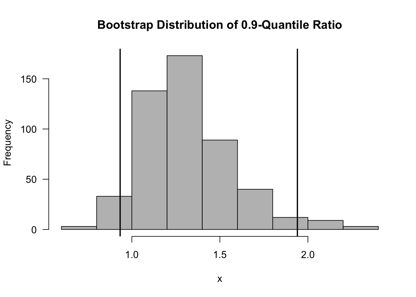
Figure 9.1: Bootstrap Distribution of the 0.9-Quantile Ratio. Vertical Lines are the Upper and Lower Bounds from the Percentile Bootstrap Confidence Interval.

9.2.3.1 Comparing the Performance of the Bootstrap and Large-Sample Confidence Intervals

• We just saw that the bootstrap and the large-sample confidence intervals gave different answers.

• For this problem, what is the best approach for constructing confidence intervals?

• We can compare the performance of different confidence intervals by looking at their coverage probability.

• For a vector of data \(\mathbf{X} = (X_{1}, \ldots, X_{n})\), we can represent a confidence interval for a parameter of interest \(\theta\) as \[\begin{equation} \Big[ L_{\alpha}(\mathbf{X}), U_{\alpha}(\mathbf{X}) \Big] \end{equation}\]
  • \(L_{\alpha}(\mathbf{X})\) is the lower confidence bound.
  • \(U_{\alpha}( \mathbf{X} )\) is the upper confidence bound.

• The coverage probability of a confidence interval \([ L_{\alpha}(\mathbf{X}), U_{\alpha}(\mathbf{X})]\) is \[\begin{equation} P\Big( L_{\alpha}(\mathbf{X}) \leq \theta \leq U_{\alpha}(\mathbf{X}) \Big), \nonumber \end{equation}\] where we usually construct \(L_{\alpha}(\mathbf{X})\) and \(U_{\alpha}(\mathbf{X})\) so that the coverage probability is exactly equal or close to \(1 - \alpha\).

• We can estimate this probability via simulation by looking at the following coverage proportion \[\begin{equation} \textrm{CoverProp}_{n_{rep}}(\theta) = \frac{1}{n_{rep}}\sum_{k=1}^{n_{rep}} I\Big( L_{\alpha}(\mathbf{X}^{(k)}) \leq \theta \leq U_{\alpha}(\mathbf{X}^{(k)}) \Big) \nonumber \end{equation}\]
  • \(n_{rep}\) is the number of simulation replications
  • \(X^{(k)}\) is the dataset from the \(k^{th}\) simulation replication
  • Each dataset \(X^{(k)}\) is generated under the assumption that \(\theta\) is the true value of the parameter of interest.

---

• We will compare coverage proportions using the same simulation design we used before for this quantile ratio example.

• That is, \(p = 0.9\) and \(X_{i} \sim \textrm{Gamma}(2, 1.5)\) and \(Y_{i} \sim \textrm{Gamma}(2, 2)\) with \(n = 100\) and \(m = 100\).

• Below shows code for a simulation study which uses 1000 simulation replications. It compares the large-sample confidence interval which uses (9.4) with two bootstrap confidence intervals.

n <- 100
m <- 100
R <- 500
eta.true <- 4/3

nreps <- 1000
Cover.par.ci <- numeric(nreps)
Cover.bootsd.ci <- numeric(nreps)
Cover.bootquant.ci <- numeric(nreps)
for(k in 1:nreps)  {
    ## Step 1: Generate the Data from Two Groups
    xx <- rgamma(n, shape=2, rate=1.5) 
    yy <- rgamma(m, shape=2, rate=2)

    ## Step 2: Estimate eta from this data
    theta.hat1 <- quantile(xx, probs=0.9)
    theta.hat2 <- quantile(yy, probs=0.9)
    eta.hat <- theta.hat1/theta.hat2    

    ## Step 3: Find confidence interval using large-sample Normal approximation
    xdensity <- density(xx)
    ydensity <- density(yy)
    fx <- approxfun(xdensity$x, xdensity$y)(theta.hat1)
    fy <- approxfun(ydensity$x, ydensity$y)(theta.hat2)
    q1.se.sq <- (.9*.1)/(n*(fx*theta.hat2)^2)
    q2.se.sq <- (.9*.1*theta.hat1*theta.hat1)/(n*fy*fy*((theta.hat2)^4))
    std.err <- sqrt(q1.se.sq + q2.se.sq)
    par.ci <- c(eta.hat - 1.96*std.err, eta.hat + 1.96*std.err)

    ## Step 4: Find bootstrap confidence intervals using R bootstrap replications
    eta.boot <- numeric(R)
    for(r in 1:R)   {
        boot.xx <- sample(xx, size=n, replace = TRUE)
        boot.yy <- sample(yy, size=m, replace = TRUE)
        thetahat.p1 <- quantile(boot.xx, probs=0.9)
        thetahat.p2 <- quantile(boot.yy, probs=0.9)
        eta.boot[r] <- thetahat.p1/thetahat.p2
    }
    boot.ci.sd <- c(eta.hat - 1.96*sd(eta.boot), eta.hat + 1.96*sd(eta.boot))
    boot.ci.quant <- quantile(eta.boot, probs=c(.025, .975))
    
    ## Step 5: Record if the true parameter is covered or not:
    Cover.par.ci[k] <- ifelse(par.ci[1] < eta.true & par.ci[2] >= eta.true, 1, 0)
    Cover.bootsd.ci[k] <- ifelse(boot.ci.sd[1] < eta.true & boot.ci.sd[2] >= eta.true, 
                                 1, 0)
    Cover.bootquant.ci[k] <- ifelse(boot.ci.quant[1] < eta.true & 
                                        boot.ci.quant[2] >= eta.true, 1, 0)
}

• The coverage proportions for each of the methods are:

mean(Cover.par.ci)

## [1] 0.921

mean(Cover.bootsd.ci)

## [1] 0.949

mean(Cover.bootquant.ci)

## [1] 0.959

• Using these simulated outcomes, we can also construct \(95\%\) confidence intervals for the coverage probabilities:

Estimates and Confidence Intervals for the Coverage Probabilities of Different Methods.

	Lower CI	Estimate	Upper CI
Large-Sample Approximation	0.904	0.921	0.938
Bootstrap Std. Err.	0.935	0.949	0.963
Bootstrap Percentile	0.947	0.959	0.971

9.3 Why is the Bootstrap Procedure Reasonable?

• As mentioned before, our original motivation for the bootstrap was to find an estimate of \(\textrm{Var}(T_{n})\) where \(T_{n}\) is a statistic that can be thought of as an estimate of \(\theta\).

• The statistic \(T_{n}\) can be thought of as a function of our sample \[\begin{equation} T_{n} = h(X_{1}, \ldots, X_{n}) \nonumber \end{equation}\] where \(X_{1}, \ldots, X_{n}\) is an i.i.d. sample with cumulative distribution function \(F\).

• If we had a way of simulating data \(X_{i}^{(k)}\) from \(F\), we could estimate \(\textrm{Var}(T_{n})\) with the following quantity \[\begin{eqnarray} \widehat{\textrm{Var}( T_{n} )} &=& \frac{1}{K-1}\sum_{k=1}^{K}\Big( h(X_{1}^{(k)}, \ldots, X_{n}^{(k)}) - \frac{1}{K}\sum_{k=1}^{K} h(X_{1}^{(k)}, \ldots, X_{n}^{(k)}) \Big)^{2} \nonumber \\ &=& \frac{1}{K-1}\sum_{k=1}^{K}\Big( T_{n}^{(k)} - \frac{1}{K}\sum_{k=1}^{K} T_{n}^{(k)} \Big)^{2} \tag{9.5} \end{eqnarray}\]
  • \(X_{1}^{(k)}, \ldots, X_{n}^{(k)}\) is an i.i.d. sample from \(F\).
  • \(T_{n}^{(k)} = h(X_{1}^{(k)}, \ldots, X_{n}^{(k)})\) is the value of out statistic of interest from the \(k^{th}\) simulated dataset.

---

• In practice, \(F\) is unknown, and we cannot simulate data from \(F\).

• The main idea behind the bootstrap is that the empirical distribution function \(\hat{F}_{n}\) is a very good estimate of \(F\).

• Hence, if we sample \(X_{1}^{(k)}, \ldots, X_{n}^{(k)}\) from \(\hat{F}_{n}\) instead of \(F\) and use the formula (9.5), this should give us a good estimate of the variance of \(T_{n}\).

---

• How can we simulate data from \(\hat{F}_{n}\)?

• Recall that \(\hat{F}_{n}\) is a discrete distribution that has mass \(1/n\) at each of the observed data points \(\mathbf{X} = (X_{1}, \ldots, X_{n})\).

• So, if we say \(X_{i}^{*} \sim \hat{F}_{n}\), then \[\begin{equation} P( X_{i}^{*} = X_{j}) = 1/n \qquad \textrm{ for } j=1,\ldots,n, \end{equation}\] where \((X_{1}, \ldots, X_{n})\) can be thought of as fixed numbers.

• To simulate a random variable \(X_{i}^{*} \sim \hat{F}_{n}\), we just need to draw one of the observations \(X_{j}\) from \(\mathbf{X}\) at random and set \(X_{i}^{*} = X_{j}\).

• Then, to simulate an i.i.d. sample \(X_{1}^{*}, \ldots, X_{n}^{*}\) from \(\hat{F}_{n}\), we just to sample the \(X_{i}^{*}\) from \(\mathbf{X}\) with replacement. In other words, we just need to use the same procedure we discussed earlier for generating bootstrap samples.

• Each bootstrap sample \((X_{1}^{*}, \ldots, X_{n}^{*})\) can be thought of as an i.i.d. sample from \(\hat{F}_{n}\).

---

• The variance of \(T_{n}\) can be written as \[\begin{equation} V_{T_{n}}(F) = \int \cdots \int h^{2}(x_{1}, \ldots, x_{n}) dF(x_{1})\cdots dF(x_{n}) - E_{T_{n}}^{2}(F), \nonumber \end{equation}\] where \[\begin{equation} E_{T_{n}}(F) = \int \cdots \int h(x_{1}, \ldots, x_{n}) dF(x_{1})\cdots dF(x_{n}), \nonumber \end{equation}\]

• What we are trying to compute with the bootstrap is the following variance estimate \[\begin{equation} V_{T_{n}}(\hat{F}_{n}) = \int \cdots \int h^{2}(x_{1}, \ldots, x_{n}) d\hat{F}_{n}(x_{1})\cdots d\hat{F}_{n}(x_{n}) - E_{T_{n}}^{2}(\hat{F}_{n}) \tag{9.6} \end{equation}\]

• It is too difficult to compute (9.6) in most cases. Instead, with the bootstrap, we are approximating (9.6) via simulation by drawing many i.i.d. samples from \(\hat{F}_{n}\).

• You can think of the bootstrap as using Monte Carlo integration to approximate (9.6).

---

• There are cases where the bootstrap does not really work well.

• The main requirement for the bootstrap to work is that the functional \(E_{T_{n}}(F)\) is “smooth” as \(F\) varies.

• That is, if \(F_{1}\) and \(F_{2}\) are “close”, then \(E_{T_{n}}(F_{1})\) and \(E_{T_{n}}(F_{2})\) should also be close.

• More specifically, if the functional \(E_{T_{n}}(F)\) is differentiable in an appropriate sense, then confidence intervals from the bootstrap estimate of the variance of \(T_{n}\) will be “valid” in an asymptotic sense (see, for example, Chapter 5 of Shao (2003) for a somewhat more rigorous discussion of this).

9.4 Pivotal Bootstrap Confidence Intervals

• Confidence intervals are often based on what is referred to as a pivot.

• The quantity \(W_{n}( \mathbf{X}, \theta)\) is a pivot if the distribution of \(W_{n}(\mathbf{X}, \theta)\) does not depend on \(\theta\).

• A common example of this is for the \(\textrm{Normal}(\theta, \sigma^{2})\) distribution. In this case, \[\begin{equation} W_{n}(\mathbf{X}, \theta) = \bar{X} - \theta \end{equation}\] is a pivot. The distribution of \(W_{n}(\mathbf{X}, \theta)\) is \(\textrm{Normal}(0, \sigma^{2})\).

• Using the pivot allows us to construct a confidence interval because \[\begin{eqnarray} 1 - \alpha &=& P\Big( -\sigma z_{1 - \alpha/2} \leq W_{n}(\mathbf{X}, \theta) \leq \sigma z_{1 - \alpha/2} \Big) \nonumber \\ &=& P\Big(-\sigma z_{1 - \alpha/2} \leq \bar{X} - \theta \leq \sigma z_{1 - \alpha/2} \Big) \nonumber \\ &=& P\Big(\bar{X} - \sigma z_{1 - \alpha/2} \leq \theta \leq \bar{X} + \sigma z_{1 - \alpha/2} \Big) \nonumber \end{eqnarray}\]

• Another common pivot (if we did not assume \(\sigma^{2}\) was known) would be \[\begin{equation} W_{n}(\mathbf{X}, \theta) = \frac{\sqrt{n}(\bar{X} - \theta)}{\hat{\sigma}}, \nonumber \end{equation}\] which would have a \(t\) distribution.

---

• We can use a similar idea to construct a bootstrap confidence interval for \(\theta = E( T_{n} )\).

• Assume that \(W_{n}(\mathbf{X}, \theta) = T_{n} - \theta\) is a pivot and suppose that \(H(t)\) is the cdf of this pivot

• Then, if we choose \(b > a\) such that \(H(b) - H(a) = 1 - \alpha\), \[\begin{eqnarray} 1 - \alpha &=& P\Big( a \leq T_{n} - \theta \leq b) = P\Big( -b \leq \theta - T_{n} \leq -a \Big) \nonumber \\ &=& P\Big(T_{n} -b \leq \theta \leq T_{n} -a \Big) \nonumber \end{eqnarray}\] For example, \(b = H^{-1}(1 - \alpha/2)\) and \(a = H^{-1}(\alpha/2)\) would work.

• This would suggest that \([T_{n} - b, T_{n} - a]\) should be a good confidence interval for \(\theta\).

• The only problem is that \(H(t)\) is not known. So, how do we find \(a\) and \(b\) if we don’t assume normality of \(T_{n}\) and a known \(\sigma^{2}\)?

• Look at the distribution of \(T_{n,r}^{*} - T_{n}\) as a substitute for \(T_{n} - \theta\) and use the empirical distribution function of \(T_{n,r}^{*} - T_{n}\) to estimate \(H(t)\) \[\begin{equation} \hat{H}_{R}(t) = \frac{1}{R}\sum_{r=1}^{R} I\Big(T_{n,r}^{*} - T_{n} \leq t \Big) \end{equation}\]

• Using this approximation for \(H(t)\), we could use the following confidence interval \[\begin{equation} \Big[ T_{n} - \hat{H}_{R}^{-1}(1 - \alpha/2), T_{n} - \hat{H}_{R}^{-1}(\alpha/2) \Big] \nonumber \end{equation}\]

---

Studentized Bootstrap Confidence Intervals

• Now, suppose we instead use the pivot \[\begin{equation} \mathbf{Z}_{n}(\mathbf{X}, \theta) = \frac{T_{n} - \theta}{se_{boot}}, \nonumber \end{equation}\] where \(se_{boot}\) denotes the bootstrap estimate of standard error.

• We will let \(K(t)\) denote the cdf of \(\mathbf{Z}_{n}( \mathbf{X}, \theta)\).

• Using the same reasoning as before, \[\begin{eqnarray} 1 - \alpha &=& P\Big( K^{-1}(\alpha/2) \leq \frac{T_{n} - \theta}{se_{boot}} \leq K^{-1}(1 - \alpha/2) \Big) \nonumber \\ &=& P\Big( - se_{boot} \times K^{-1}(1 - \alpha/2) \leq \theta - T_{n} \leq -se_{boot} \times K^{-1}(\alpha/2) \Big) \nonumber \\ &=& P\Big(T_{n} - se_{boot} \times K^{-1}(1 - \alpha/2) \leq \theta \leq T_{n} - se_{boot} \times K^{-1}(\alpha/2) \Big) \nonumber \end{eqnarray}\] and hence a confidence interval for \(\theta\) would be \[\begin{equation} \Big[ T_{n} - se_{boot} \times K^{-1}(1 - \alpha/2), T_{n} - se_{boot} \times K^{-1}(\alpha/2) \Big] \nonumber \end{equation}\]

• To estimate \(K(t)\), we are going to use \(Z_{n,r}^{*} = (T_{n,r}^{*} - T_{n})/\hat{se}_{r}\) as a substitute for \((T_{n} - \theta)/se_{boot}\).

• The estimate \(\hat{se}_{r}\) is an estimate of the standard error of \(T_{n,r}^{*}\). This could be estimated via \[\begin{equation} \hat{se}_{r} = \Bigg[ \frac{1}{J-1} \sum_{j=1}^{J} \Big( T_{n,r,j}^{**} - \frac{1}{J} \sum_{j=1}^{J} T_{n,r,j}^{**} \Big)^{2} \Bigg]^{1/2}, \nonumber \end{equation}\] where \(T_{n,r,j}^{**}\) is the value of our test statistic computed from the \(j^{th}\) bootstrap sample of the bootstrap sample that was used to produce \(T_{n,r}^{*}\).

• So, to find \(\hat{se}_{r}\), we need \(J\) bootstrap samples within each of the \(R\) bootstrap samples that were used to generated \(T_{n,1}^{*}, \ldots, T_{n,R}^{*}\). For this reason, this is often referred to as the double bootstrap.

• Then, the estimate of \(K(t)\) is defined as \[\begin{equation} \hat{K}_{R}(t) = \frac{1}{R} \sum_{r=1}^{R} I\Big( Z_{n,r}^{*} \leq t \Big) \nonumber \end{equation}\]

• The studentized bootstrap confidence interval (or the bootstrap-t confidence interval) is then defined as \[\begin{equation} \Big[ T_{n} - se_{boot} \times \hat{K}_{R}^{-1}(1 - \alpha/2), T_{n} - se_{boot} \times \hat{K}_{R}^{-1}(\alpha/2) \Big] \nonumber \end{equation}\]

9.5 The Parametric Bootstrap

• With the bootstrap, we generate each bootstrap sample \((X_{1}^{*}, \ldots, X_{n}^{*})\) by sampling with replacement from the empirical distribution function \(\hat{F}_{n}\).

• For this reason, it can be referred to as the nonparametric bootstrap.

• With the parametric bootstrap, we sample from a parametric estimate \(F_{\hat{\varphi}}\) of the cumulative distribution function instead of sampling from \(\hat{F}_{n}\).

• For example, suppose we have data \((X_{1}, \ldots, X_{n})\) that we assume are normally distributed and we estimate \(\mu\) and \(\sigma^{2}\) with \[\begin{equation} \hat{\mu} = \bar{X} \qquad \qquad \hat{\sigma}^{2} = \frac{1}{n-1}\sum_{i=1}^{n} (X_{i} - \bar{X})^{2} \end{equation}\]

• If we are interested in getting a confidence interval for \(\theta\) where \(T_{n} = h(X_{1}, \ldots, X_{n})\) is an estimate of \(\theta\), the parametric bootstrap would use the following procedure:

• For \(r = 1, \ldots, R\):
  • Draw an i.i.d. sample: \(X_{1}^{*}, \ldots, X_{n}^{*} \sim \textrm{Normal}(\hat{\mu}, \hat{\sigma}^{2})\).
  • Compute \(T_{n,r}^{*} = h(X_{1}^{*}, \ldots, X_{n}^{*})\).

• Then, form a confidence interval for \(\theta\) using the parametric bootstrap replications \(T_{n,1}^{*}, \ldots, T_{n,R}^{*}\)

---

When Might the Parametric Bootstrap be Useful?

• In cases with smaller sample sizes. For small sample sizes, \(F_{\hat{\varphi}}\) is often a better estimate than \(\hat{F}_{n}\).

• When you are only interested in constructing a confidence interval for the parameter of a parametric model that you think fits the data well.

• For non-i.i.d. data or other complicated distributions, a parametric bootstrap can sometimes be easier to work with.

---

• For non-i.i.d. data, where our observations \((X_{1}, \ldots, X_{n})\) our dependent, a parametric bootstrap can often be straightforward to implement.

• Suppose \(G_{\varphi}\) is a parametric model that describes the joint distribution of \((X_{1}, \ldots, X_{n})\) and that it is easy to simulate observations from \(G_{\varphi}\).

• Then, if you have an estimate \(\hat{\varphi}\) of \(\varphi\), you can use the following procedure to generate bootstrap replications for your statistic of interest.

• For \(r = 1, \ldots, R\):
  • Draw a sample \((X_{1}^{*}, \ldots, X_{n}^{*}) \sim G_{\hat{\varphi}}\).
  • Compute \(T_{n,r}^{*} = h(X_{1}^{*}, \ldots, X_{n}^{*})\).

9.5.1 Parametric Bootstrap for the Median Age from the Kidney Data

• Let us consider the ages from the kidney data.

• One somewhat reasonable model for the ages \(X_{i}\) from the kidney data is that \[\begin{equation} X_{i} - 17 \sim \textrm{Gamma}(\alpha, \beta) \nonumber \end{equation}\]

• We can find the maximum likelihood estimates \((\hat{\alpha}, \hat{\beta})\) for this model using the following R code

kidney <- read.table("https://web.stanford.edu/~hastie/CASI_files/DATA/kidney.txt", 
                     header=TRUE)

LogProfLik <- function(alpha, x) {
    ans <- alpha*log(alpha/mean(x)) - lgamma(alpha) + (alpha - 1)*mean(log(x)) - alpha
    return(ans)
}

best.alpha <- optimize(LogProfLik, interval=c(0,10), x=kidney$age - 17, 
                       maximum=TRUE)$maximum
best.beta <- best.alpha/mean(kidney$age - 17)

• We can plot this estimated Gamma density overlaid on the histogram of the ages to see how they compare

tt <- seq(17, 90, length.out=500)
hist(kidney$age, breaks="FD", probability=TRUE, las=1, xlab="Age", 
     main="Estimate Gamma Density for the Kidney Age Data", col="grey")
lines(tt, dgamma(tt - 17, shape=best.alpha, rate=best.beta), lwd=2)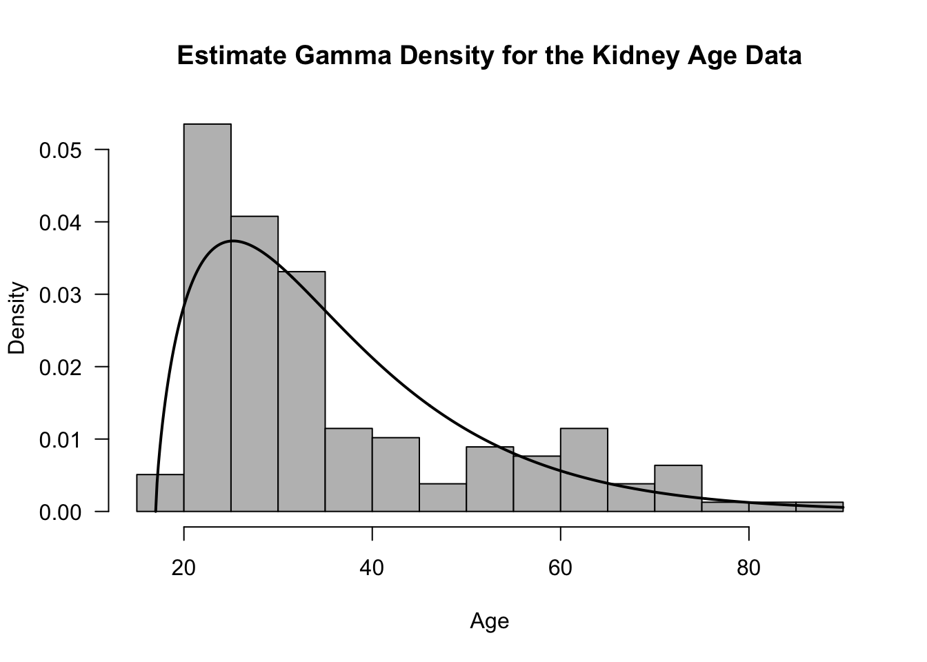

---

• Suppose we are interested in constructing a confidence interval for the median age.

• To use the parametric boostrap with the parametric model \(X_{i} - 17 \sim \textrm{Gamma}(\alpha, \beta)\) and using our estimates \(\hat{\alpha}\) and \(\hat{\beta}\) computed above, we would use the following steps.

• For \(r = 1, \ldots, R\):
  • Draw an i.i.d. sample: \(X_{1}^{*}, \ldots, X_{n}^{*} \sim 17 + \textrm{Gamma}(\hat{\alpha}, \hat{\beta})\).
  • Compute \(T_{n,r}^{*} = \textrm{median}(X_{1}^{*}, \ldots, X_{n}^{*})\).

• The code for implementing this parametric bootstrap is given below

R <- 500
med.boot.par <- rep(0, R)
med.boot.np <- rep(0, R)
for(r in 1:R) {
    xx.boot.par <- 17 + rgamma(157, shape=best.alpha, rate=best.beta)
    xx.boot.np <- sample(kidney$age, size=157, replace=TRUE)
    
    med.boot.par[r] <- median(xx.boot.par)  ## rth par. bootstrap replication
    med.boot.np[r] <- median(xx.boot.np)  ## rth par. bootstrap replication
}

• The normal standard error confidence interval using the parametric bootstrap is

c(median(kidney$age) - 1.96*sd(med.boot.par), median(kidney$age) + 1.96*sd(med.boot.par))

## [1] 28.39858 33.60142

• The normal standard error confidence interval using the nonparametric bootstrap is

c(median(kidney$age) - 1.96*sd(med.boot.np), median(kidney$age) + 1.96*sd(med.boot.np))

## [1] 28.64083 33.35917

9.6 Additional Reading

• Additional reading which covers the material discussed in this chapter includes:
  • Chapter 3 from Wasserman (2006)
  • Chapter 2 from Davison and Hinkley (1997)

9.7 Exercises

• Exercise 9.1 With the regular bootstrap we generate bootstrap samples by sampling from the empirical distribution function \(\hat{F}_{n}\). An alternative approach is to sample from a smooth estimate of \(F\) instead of the non-smooth estimate \(\hat{F}_{n}\). Consider the following smooth estimate of \(F\) which is just the indefinite integral of a kernel density estimate \[\begin{equation} \hat{F}_{h}^{KD}(t) = \frac{1}{n} \sum_{i=1}^{n} \int_{-\infty}^{t} \frac{1}{h} K\Big( \frac{x - X_{i}}{h} \Big) dx \nonumber \end{equation}\]

• What is \(\hat{F}_{h}^{KD}\) when \(K( \cdot )\) is the Gaussian kernel?
• For the case of a Gaussian kernel, how do you generate an i.i.d. sample \((X_{1}^{*}, \ldots, X_{n}^{*})\) from \(\hat{F}_{h}^{KD}\)?
• Using the dataset from the package, compute a \(95\%\) ``smooth bootstrap" confidence interval for the standard deviation \(\sigma_{v}\) of the velocities by using the following steps: For \(r = 1,\ldots, R\):
  • Draw an i.i.d. sample: \(X_{1}^{*}, \ldots, X_{n}^{*} \sim \hat{F}_{h}^{KD}\).
  • Compute \(T_{n,r}^{*} = \textrm{sd}( X_{1}^{*}, \ldots, X_{n}^{*})\).

• Using \(T_{n,1}^{*}, \ldots, T_{n,R}^{*}\), construct the confidence interval for \(\sigma_{v}\) using the normal bootstrap standard error approach. For the bandwidth \(h\) in \(\hat{F}_{h}^{KD}\), you can use Silverman’s rule-of-thumb: \(h = 0.9 n^{-1/5}\min\{ \hat{\sigma}, IQR/1.34 \}\).

• Using the usual bootstrap where we sample from \(\hat{F}_{n}\), construct three \(95\%\) bootstrap confidence intervals for \(\sigma_{v}\) using the following methods
  • Normal bootstrap standard error confidence interval.
  • A pivotal bootstrap confidence interval based on \(T_{n,r}^{*} - T_{n}\) (not the studentized bootstrap confidence interval).
  • Bootstrap percentile confidence interval.

References

Davison, Anthony Christopher, and David Victor Hinkley. 1997. Bootstrap Methods and Their Application. Vol. 1. Cambridge university press.

Shao, Jun. 2003. Mathematical Statistics. 2nd ed. Springer-Verlag New York Inc.

Wasserman, Larry. 2006. All of Nonparametric Statistics. Springer Science & Business Media.